TL;DR: We present details of our distributed training codebase, known as Titan. Titan provides several close-to-the-hardware tricks, optimizations, and logging facilities for large scale foundation model training. We then discuss how we use Titan as part of the Model Factory to conduct architectural experimentation at scale, and we conclude with a discussion of how we reliably train large foundation models across our 10K GPU cluster.
Introduction
In our previous post, we discussed Poolside's data stack, ranging from data ingestion through to producing data blends. Now that we've covered all of those details, we can now dig into the furnaces of our Model Factory: our pre-training codebase, named Titan.
In today's post, we'll look at the philosophy behind our pre-training codebase. In particular, we’ll begin by discussing how our Titan codebase came to be, including a discussion of our previous pre-training codebase. We’ll then move onto how we used these insights to design Titan as a flexible and performant pre-training codebase. Next, we’ll discuss how we use Titan as part of the Model Factory to conduct architectural experiments at scale. Finally, we’ll wrap up by discussing how we reliably train and automatically evaluate large foundation models at scale across our 10K GPU cluster.
How we decided on Titan
Before we dig too much into how Titan works, it’s worth describing how Titan came to be. After all, it's rare that you get things right the first time around.
Although we now have a fully functioning Factory for training models and running architectural experiments, this wasn’t always the case. In fact, when Poolside was founded in April 2023, we had an entirely different set of concerns compared to today. For one thing, our compute budget was orders of magnitude smaller than it is today; our first training cluster consisted of just a few nodes equipped with A100 GPUs. At the same time, we had a small team: our Foundations team consisted of only three engineers until the early part of 2024, when it quickly began to grow.
When you’re only training on a few nodes, your priorities look very different compared to your priorities when you have 10K GPUs. You really need to prioritize the ability to debug training at a moment’s notice, and really pay close attention to the low-level details of what’s happening during training. In fact, because we had comparatively few GPUs, we typically only had a few GPU jobs running in parallel at once, making monitoring relatively easy. We were also very concerned about memory limits. We knew that we wanted to experiment with models of different sizes, and we didn’t want to prematurely limit our ability to conduct these experiments.
These constraints presented us with a problem: we could either adapt a large, open-source training framework to fit our needs, or we could write everything from scratch. In the end, we took a hybrid approach: we built an internal distributed pre-training codebase, called Monster, using a mixture of PyTorch and other open source libraries. In some places, we manually wrapped and forked low-level libraries, such as Xformers, libtorch and NCCL; and, in other places, we implemented our own CUDA and Triton kernels. With the constraints that we had at the time, building Monster was the right decision, and those of us who worked on it still retain fond memories of building our very own Monster from the ground up.
But after a while, Monster began to stagger. Looking back, pressure on Monster arrived from four distinct directions. First, our constraints and priorities changed as time went on. Where before we only had a few jobs running in parallel, we suddenly found ourselves executing hundreds of jobs in parallel. At this scale, debugging individually failing jobs becomes substantially less viable without proper tooling. Additionally, we were struggling to keep up with the outside world: almost every feature we wanted, we had to build ourselves. More pressingly, we found that we were falling behind: our optimizations were not as good as those in the outside world, primarily because of how we’d built Monster. Specifically, early on we designed Monster around the use of pipeline parallelism, and the inflexibility of our design meant that Monster creaked whenever we needed to add new features. In a sense, this inflexibility was a result of chasing every optimization. We made individual pieces of Monster incredibly performant, but in doing so we made the code very rigid and inflexible. Intuitively speaking, this was a consequence of Amdahl’s law []: we had lots of code that performed excellently on microbenchmarks, but ultimately this code didn’t contribute much to the overall runtime of our pre-training jobs. What’s more, the carefully optimized code prevented us from implementing wider ranging optimizations, restricting our ability to make wide-scale changes. Additionally, having a fully custom pre-training codebase presents a large onboarding challenge. A large and complicated codebase is always tricky to interpret, and we realized that we were spending a lot of time debating over terminology and layout. And, for all of its performance, Monster was still highly opinionated, making extension difficult. It simply wasn't well-suited for use in the Model Factory.
We began to look at what we could do differently. Coincidentally, TorchTitan was published around the same time we began to look for alternatives to Monster. For the unaware, TorchTitan is an open-source project that makes broad use of various PyTorch features to provide an efficient and simple template for distributed training. Notably for us, TorchTitan is written and maintained by the PyTorch team, meaning that improvements to the core of PyTorch are very usable inside TorchTitan. While we had implemented some of these improvements ourselves inside Monster, we soon realized that TorchTitan would allow us to train new models much more efficiently than we could with Monster. What’s more, we also realized that TorchTitan had the ability to provide us with a level of flexibility that we simply couldn’t match with our Monster implementation. After some initial experimentation, we decided to retire Monster in favor of a new codebase on top of TorchTitan, dubbed Titan.
So, what does Titan give us that Monster didn’t? First, with Titan we are always able to keep up with the open-source world: TorchTitan is a highly active open-source project, and we benefit tremendously from upstream innovations in both Torch and TorchTitan. These upstream innovations not only allow us to focus our time on implementing other features that we use as part of the Model Factory, but they also allow us to focus on running architectural experiments and improving the broader usability of the Model Factory. Additionally, using a PyTorch-native library makes onboarding much easier: engineers that are familiar with PyTorch already find it much easier to learn how to use Titan. And, above all, Titan is flexible enough to give us a playground for trying new ideas and optimizations, further allowing us to push the frontier of AI.
How is Titan structured?
Now that we know how Titan came to be, we can look at what it offers and how it’s structured.
First, it's important to note that Titan is not a complete rewrite from Monster. Quite the opposite. When we started building Titan, we migrated all of the Monster code into a sub-directory of our new Titan repository. Then, over time, we gradually replaced certain components with more flexible equivalents from other sources. We retained various third-party dependencies, too, in situations where these were best-in-class options.
We then began to incorporate TorchTitan. As a reminder, TorchTitan provides several useful components for large-scale training, including several parallelism strategies. We also make extensive use of other components from TorchTitan, like the simple training script approach, checkpointing, and some other helpers. But we don’t blindly use these components. They don’t always suit our use case or fulfill all of our requirements. In these cases, we typically replace these components with our own custom components. This approach helps us retain the best of both worlds: we can take things from the open-source world that are useful, but we can also build new components when needed. We also still implement several new components ourselves. For instance, our entire mixture-of-experts stack is custom, and we regularly add new custom components to the rest of the codebase too.
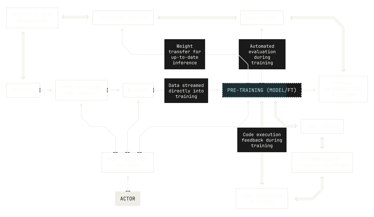
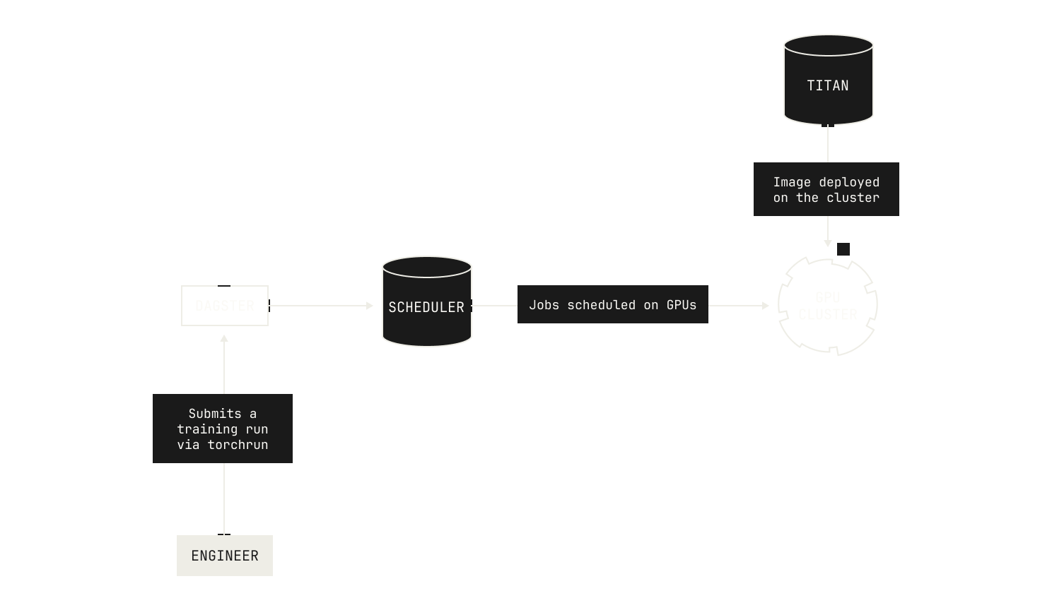
Titan itself can be used in multiple ways. In fact, Titan can be deployed across all manner of topologies: from a single machine, to our full H200 cluster and even beyond. We regularly take advantage of this flexibility when we’re implementing new features: we can experiment with new ideas and implementations on a single development node, and then we can ramp up our experiments once the feature has been sufficiently tested. It’s worth noting that a distributed pre-training codebase doesn’t exist in isolation. Indeed, running distributed pre-training jobs at scale requires multiple layers of orchestration, from node scheduling to authentication. Thankfully, Titan fits nicely into the Model Factory, and we can use primitives that we’ve built in the past to handle these concerns for us. In fact, we can deploy Titan effortlessly onto our H200 nodes via Kubernetes, and all of the node scheduling is handled for us by our orchestrator and torchrun.
We also use Titan in other ways. First of all, it’s not technically correct to refer to Titan as just a distributed pre-training codebase. Instead, Titan is a distributed training codebase; it supports supervised finetuning (SFT), various mid-training techniques, and allows us to handle various reinforcement learning workloads. We’ll discuss how we operate SFT and reinforcement learning in a future installment, but it’s worth stressing: Titan provides distributed training for every AI workload in the Model Factory.
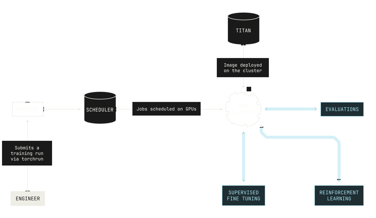
From an operational perspective, Titan can be invoked and scheduled from inside our Dagster workspace, allowing us to easily launch experiments (for more on how we use Dagster, please see the earlier posts in this series). In fact, Titan workloads can be triggered either manually—that is, via the Dagster UI—or via our continuous integration pipeline. This makes launching new experiments and training runs incredibly easy, requiring just a few clicks to get started. In fact, every Titan workload in Dagster produces a versioned Dagster asset, adding to our existing data lineage. From this perspective, our Dagster lineage acts as more than just a data lineage: it acts as a historical log of every training and data experiment we run inside the Model Factory.
Titan also serves as a dependency for other projects. As we’ve previously mentioned, Titan provides training capabilities for all manner of training and reinforcement learning workloads. But Titan can also be used explicitly as a project dependency for other projects. For instance, we use Titan as a dependency of Atlas, our inference codebase, to obtain reference results for certain parts of inference.This means that we can quickly implement new models against a known baseline: we can just use Titan's implementation of a forward pass, build an inference-specific implementation of the model, and then check that they match. The ability to check equivalences in this setting is very useful, especially when we end up employing optimizations.
Training with Titan
While a state-of-the-art pre-training codebase is a wonderful thing to have on paper, building such a codebase is an expensive and time-consuming process. As a result, it only makes sense to have such a codebase if doing so actually enables us to successfully produce high-quality foundation models. Thus, in this section we’ll discuss how we use Titan to run large-scale architectural experiments and how Titan enables us to successfully train foundation models at production-scale.
Architectural experiments
Before we get into architectural experiments, it's worth recapping why we view such experiments as mandatory for successful large-scale training.
Training a large-scale foundation model is an extremely time consuming and costly endeavor; there are only a handful of companies in the world that truly pre-train large-scale foundation models from scratch. Production-scale runs typically require many thousands of GPUs for weeks and months at a time, and every hour counts. Given this expense, we would ideally know ahead of time that the expense is worth it (i.e. that we will actually end up with a good foundation model after training has finished). More broadly, training a "good" model is a product of carefully balancing many distinct tradeoffs. On the one hand, we could train an extremely large model that would perform excellently on downstream benchmarks, but the cost and time required to build such a model may simply be too onerous. On the other hand, it's easy to train a small model cheaply, but the downstream performance on useful tasks is likely to be poor. In other words, what we're really interested in is building the best model that we can, using a fixed compute and time budget.
One way to achieve this is to establish scaling laws. Intuitively speaking, a scaling law takes a loss curve from a small model and predicts how the loss curve would change as we increase the number of parameters in the model. This is precisely what we're after: we can simply train a small model, look at the loss curve, and then predict how a larger version of the same model would perform. In the literature, this approach is referred to as hyperparameter transfer. We note that multiple approaches to hyperparameter transfer can be found in the literature, including the mu-P family of techniques. For the sake of brevity, we'll skip over the details of which techniques we use, but we stress that Titan is sufficiently flexible to accommodate multiple different hyperparameter transfer techniques in practice.
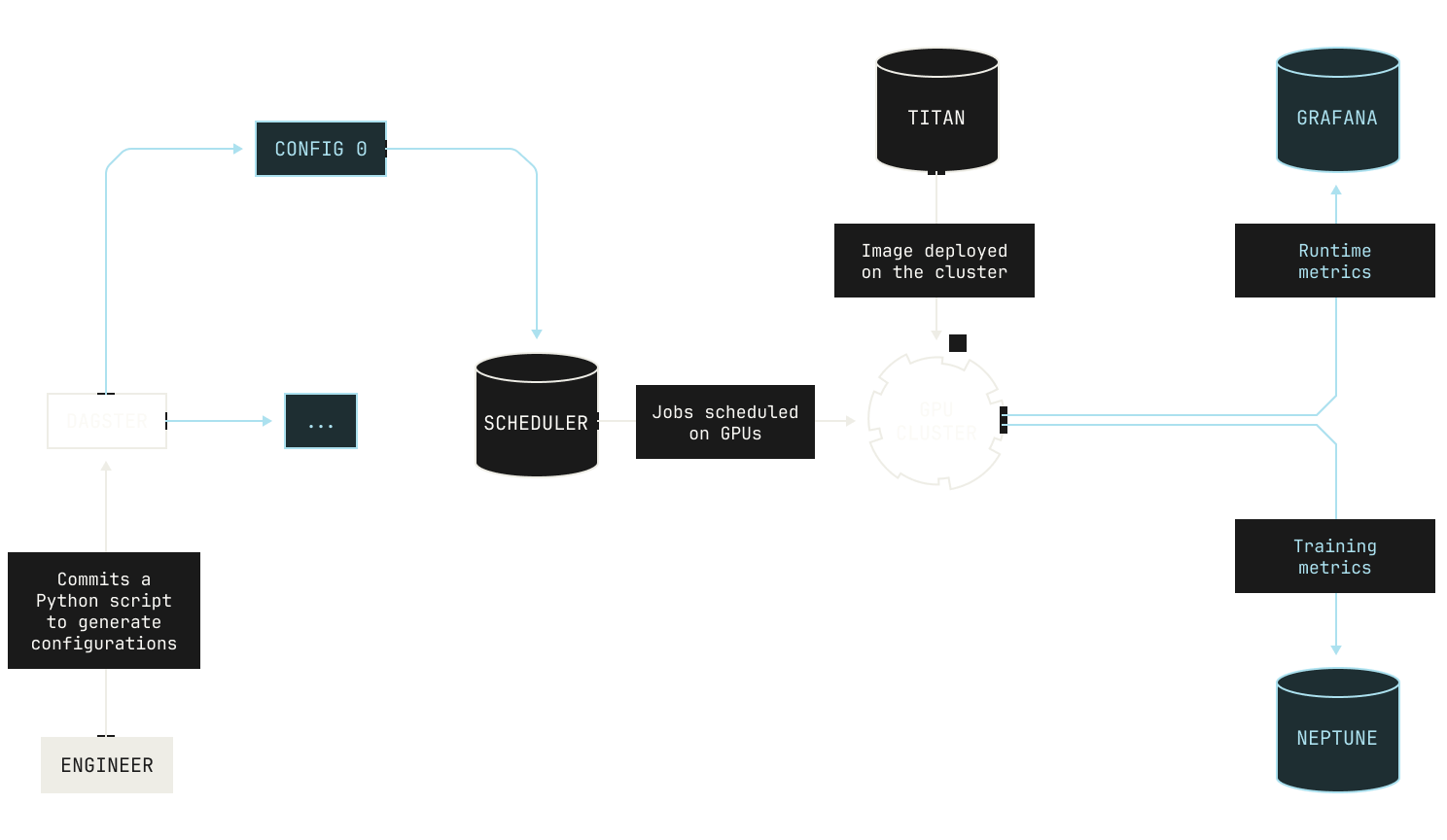
We establish scaling laws in the Model Factory in the following way. We first decide on the experiments that we want to run for a particular parameter search (or sweep), or the particular search space that we're interested in exploring. In practice, we typically end up with thousands of small experiments covering all manner of parameters, stretching across different architectural details and all manner of hyperparameters. We then write a simple Python program that produces a distinct configuration for each experiment. Then, when we launch the experiments, each configuration is registered as a versioned asset in Dagster, alongside the source code that was used to generate the particular configuration. Once a configuration is registered in Dagster, it officially becomes part of the Factory, and the real magic happens. For example, we can automatically trigger evaluations and schedule them against each of the produced checkpoints, allowing us to go beyond looking at the loss curves. Every model's metrics are also streamed directly into our Neptune dashboard, and once the experiments have concluded we ultimately look at these metrics to see which model performed the best. At the same time, we also look at the other metrics that we captured during these experiments, such as the time it takes for a single training iteration, or the peak hardware utilization that we observed during a particular model’s training run. By capturing all of this information in one place, we can more easily iterate on our architectural experiments and ultimately decide which model architecture we're going to use for a production-scale training run.
Of course, we can run other kinds of parameter sweeps in the Model Factory. For example, let’s imagine that we want to run a configuration sweep over batch sizes for a particular model architecture. As a reminder, choosing a batch size requires making a careful tradeoff: a large batch size can lead to faster training, but models can very easily get stuck in local minima during training. Small batch sizes, in contrast, can more easily escape local minima, but training is typically much slower due to lower hardware utilization.
Although we can intuitively guess at a good batch size, this is hardly a rigorous way to make such an important choice. We can inject some rigor into this process by instead running an empirical search for a good batch size. With the Model Factory, this process is almost effortless. We’ll now go into this process in detail. Just like in the previous example, we’ll start by writing a Python script that generates the configurations for us. Specifically, we’ll start by declaring a Python dictionary of potential configurations. For the sake of this example, we'll key on the number of heads, but this is not a hard restriction:
sweep_params = {
      1: {
         "batch_sizes": [(1, 8)],
         ...
      },
}
We’ll then iterate through these parameters inside a builder function. The builder function will produce a different Dagster configuration for each parameter choice.
for n_heads, config in sweep_params:
    # Create a new Dagster asset for this run
And that’s it! We can then simply open up the Dagster UI, click a few buttons, and all of the runs are immediately launched for us. Specifically, each configuration corresponds to a new pre-training run, with all of the scheduling and allocation details handled for us by the Factory. Moreover, every metric that we need will be automatically pushed to our metrics platform, allowing us to easily track how the experiments evolve over time. It’s worth noting that not every workflow follows this procedure; some workflows are triggered via our continuous integration pipeline, or via other scripts that we’ve written. But the general process—simply defining what it is we want to explore—is almost always this simple.
It’s worth highlighting how this changes the work that we do at Poolside. Before, running architectural experiments was something that we dreaded; each job required careful specification, manual deployment, and close monitoring. Now, we regularly run hundreds of experiments over a weekend, and there’s results for us to inspect first thing on Monday morning. We can even dig into these experiments: we can analyze the loss curves, look at the training logs, and derive new insights in a way that we just couldn’t before.
Production-scale pre-training
Once the experiments are out of the way, we're ready to launch a production-scale pre-training run. Remarkably, the Model Factory makes this just as easy as launching an experiment; we can simply define a configuration file that corresponds to the production-scale training job that we want to execute and launch everything in the exact same way that we do for regular experiments. It's all that simple.
There are a couple of practical differences compared to small scale experiments. First, we run automated evaluations on the checkpoints that are produced during training, sometimes as frequently as every few hundred training steps. We’ll discuss more about how we implement evaluations in a future installment of this series, but it’s worth noting that we run multiple evaluations on a model during training. Under the hood, evaluations are triggered automatically by Dagster when a new checkpoint is pushed to a particular Dagster partition. Notably, our evaluations are disaggregated and scheduled separately (i.e. we do not force all of the evaluations to run in parallel, or even at nearly the same time). This is primarily for flexibility; if our cluster is busy, we may not have capacity to run all of the evaluations in parallel. Still, once a single evaluation has finished, the evaluation’s score is pushed to Neptune, allowing us to keep track of how the model’s performance changes during training.
Although launching evaluations and training runs are easy in the Model Factory, the practice of production-scale pre-training is anything but simple. In fact, production-scale pre-training runs generally require much more care than small experimental runs. Intuitively speaking, the difference is mostly a matter of scale: because we run production-scale training on many more GPUs, there's simply more that can go wrong. For instance, GPUs fail much more frequently, loss spikes can cause training runs to be derailed, and network issues can grind training to a halt. And these issues can occur at any time: as a general rule, pre-training errors tend to trample all over sleep schedules.
In the past, we had to manually resolve these issues when they occurred, leading to many late nights and early mornings. Surely, we thought, there had to be a better way than doing this all by hand?
We tackled these problems from three different directions. First, an ounce of prevention is worth a pound of cure, and we can prevent many issues by running “pre-flight checks” on our training nodes before we launch training. Intuitively speaking, our pre-flight checks ensure that our nodes are stable for the purposes of training, and we stress test many aspects of our nodes to ensure that they’re sufficiently stable. In practice, these pre-flight checks knock out many low-hanging issues, such as broken network connections or faulty hardware. We stress that our pre-flight checks continue to evolve over time, and we continually add new tests and monitor additional metrics to ensure that everything works as expected before we start training a model.
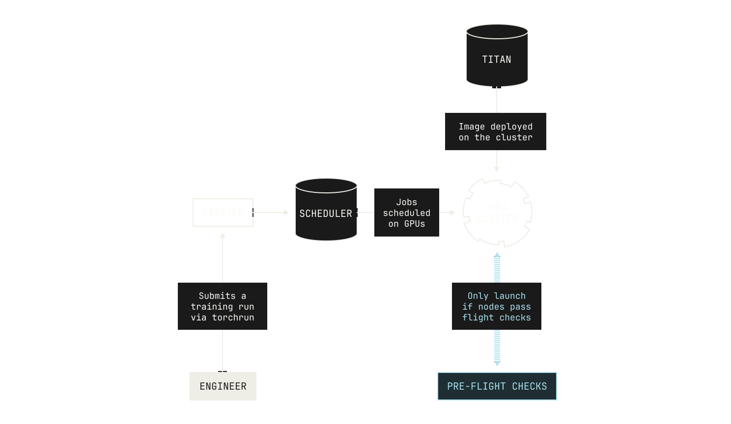
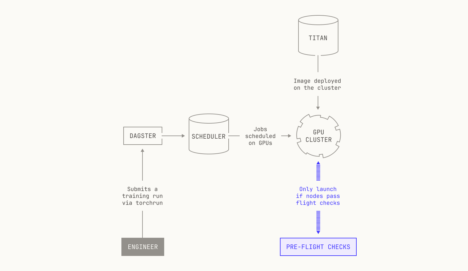
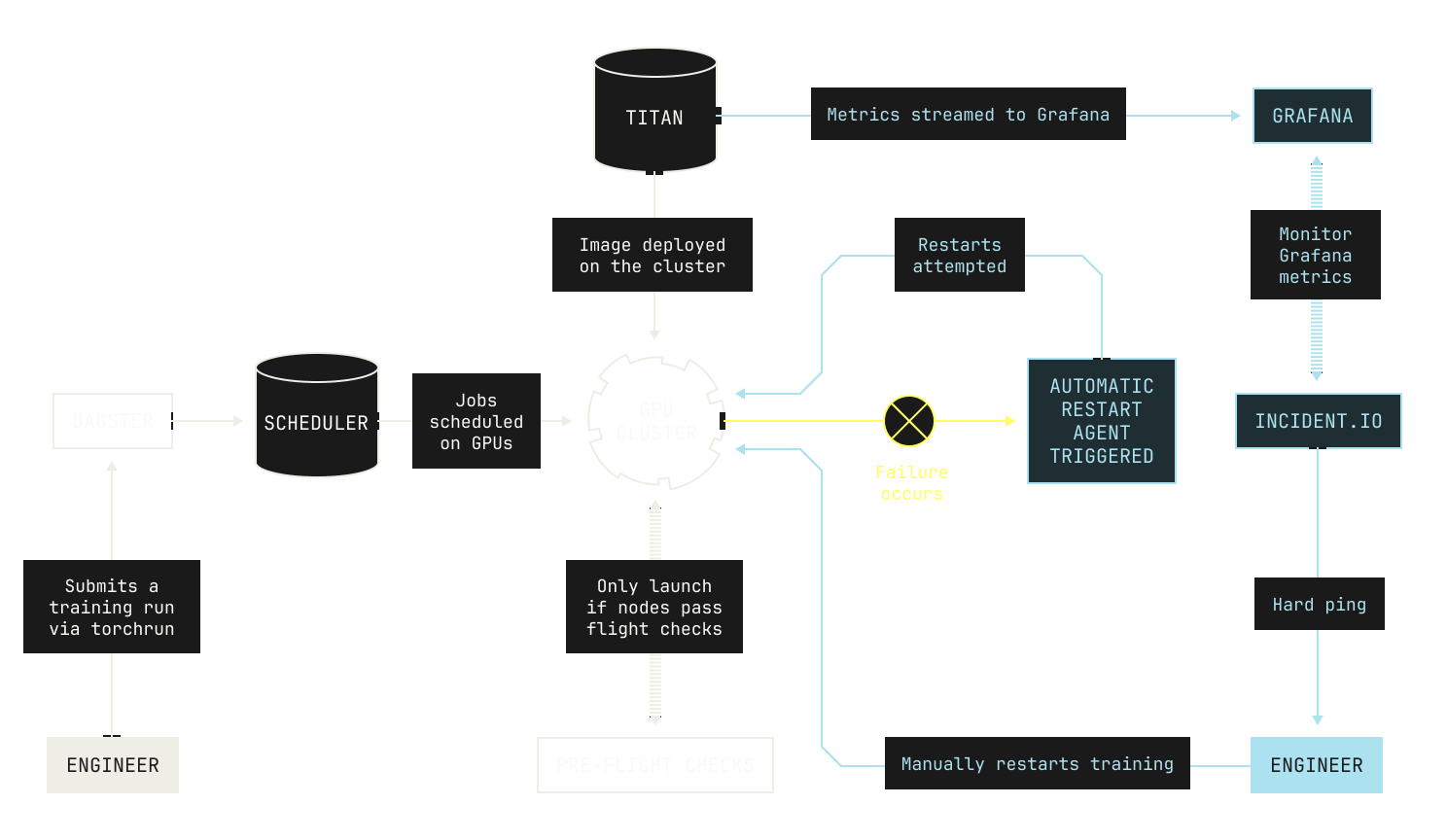
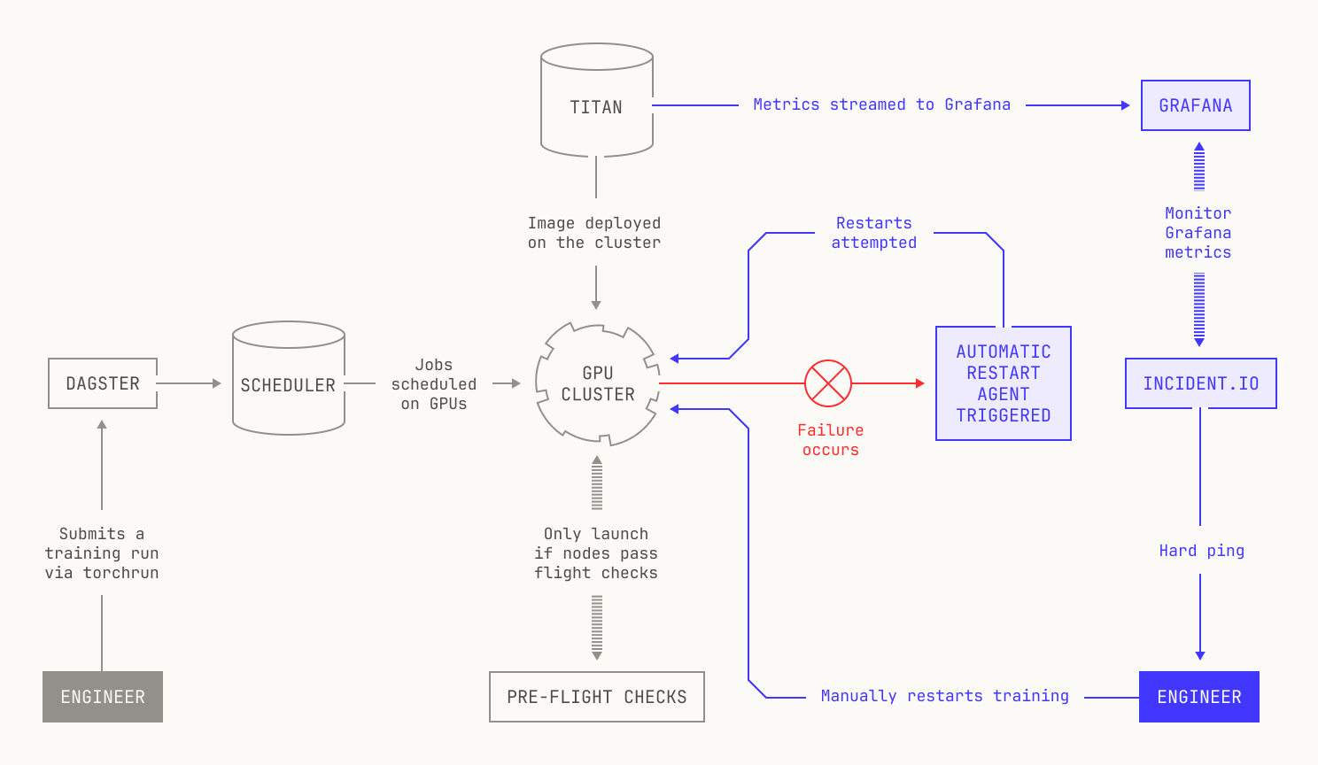
No matter what pre-flight checks we run, errors will still occur during pre-training: it’s simply inevitable at our scale. Sometimes these errors are due to programming bugs that couldn’t be captured by our pre-flight checks, such as an off-by-one error or a deadlock in a NCCL communicator. And sometimes model training just goes wrong. Loss spikes can easily occur, and chasing down the root cause of these errors requires a great deal of skill and patience. In practice, we typically diagnose these issues by using the metrics that we gather during pre-training. Moreover, Titan itself is equipped with multiple debugging facilities. We stream training logs directly into Sentry, and Titan also has support for enabling Pytorch’s FlightRecorder software, allowing us to retrospectively inspect and debug failed training runs. Lastly, we also have various proprietary tools and techniques to allow us to debug failed or poorly performing training runs in the Model Factory, allowing us to gather insights beyond those that we can get from publicly available tools.
However, directly investigating errors requires us to invest a great deal of manual effort into managing and restarting training. There is, however, a way to resolve these issues automatically without requiring our engineers to manually interact with every failed training job. It turns out that practically speaking, almost all of the error cases that happen during pre-training can be solved by following a standard working playbook. For example, let's consider the case that there's a singular faulty node that's disrupted pre-training. In the past, we would've debugged the error by first isolating the faulty node, replacing it with a known working node, and then restarting training manually. But there's no reason why this process has to be handled manually; in fact, automating this process would probably be less error prone than relying on an engineer.
To address this and other similar issues, we implemented robust automatic recovery as part of the Model Factory. Each recovery automation in the Model Factory handles a particular error case, such as a failing node. In practice, these automations kick in after training appears to be halted for a configurable period of time. Let’s say ten minutes. Notably, our automatic recovery system also incorporates automatic restarts, enabling us to quickly recover from stalled training.
Although our automated recovery handles the vast majority of error cases, there are still some rare errors that cannot be automatically recovered. In these cases, we employ a fallback system that alerts one of our engineers. In more detail, we use incident.io to monitor the metrics in our Grafana dashboard. If the incident.io service notices that no new metrics have appeared for a configurable period of time, say, thirty minutes, then incident.io will send a soft ping to our on-call engineers and to a Poolside-wide Slack channel. This soft ping is primarily to allow time for any automatic recovery procedures to complete, as automatic restarts can sometimes take a while. If training has still not recovered after a configurable period of time (say, an hour), the on-call engineers will receive a hard ping to restart. Once the ping has been acknowledged, a new Slack channel is automatically created for discussions related to the incident. Notably, this Slack channel enables us to quickly share context across engineers, leading to quicker resolutions and restarts.
Compared to manually restarting training, the quality of life improvements that automated restarts give our engineers cannot be overstated. For example, the training run for the first model produced at Poolside —Malibu v1—was an arduous, weeks-long period of near continuous babysitting and debugging. Although that experience gave rise to many important lessons about large-scale model training, our new approach gives us a level of serenity and peace of mind that simply seemed unobtainable in the days before the Model Factory.
Thank you
We hope you enjoyed reading this post about Titan and our approach to training foundation models. In our next installment, we’ll take a look into another crucial piece of the Model Factory: our code-execution platform.
Acknowledgments
We would like to thank Poolside’s foundations team for their thoughtful comments and insights on this post.