A deep dive into the Model Factory's data pipelines
TL;DR: Data is the lifeblood of foundation model training. In this post we’ll present a deep dive into our data processing pipelines and workflows, spanning our entire data workflow. In particular, we discuss the engineering behind every aspect of our data pipelines, including data ingest, synthetic data generation, filtering, deduplication, blending and streaming.
Introduction
In our previous post, we introduced the Model Factory, Poolside's internal systems framework for training foundation models at scale. Now that we understand how the Factory works at a high level, we can discuss the individual pieces of the Factory and how they all gel together.
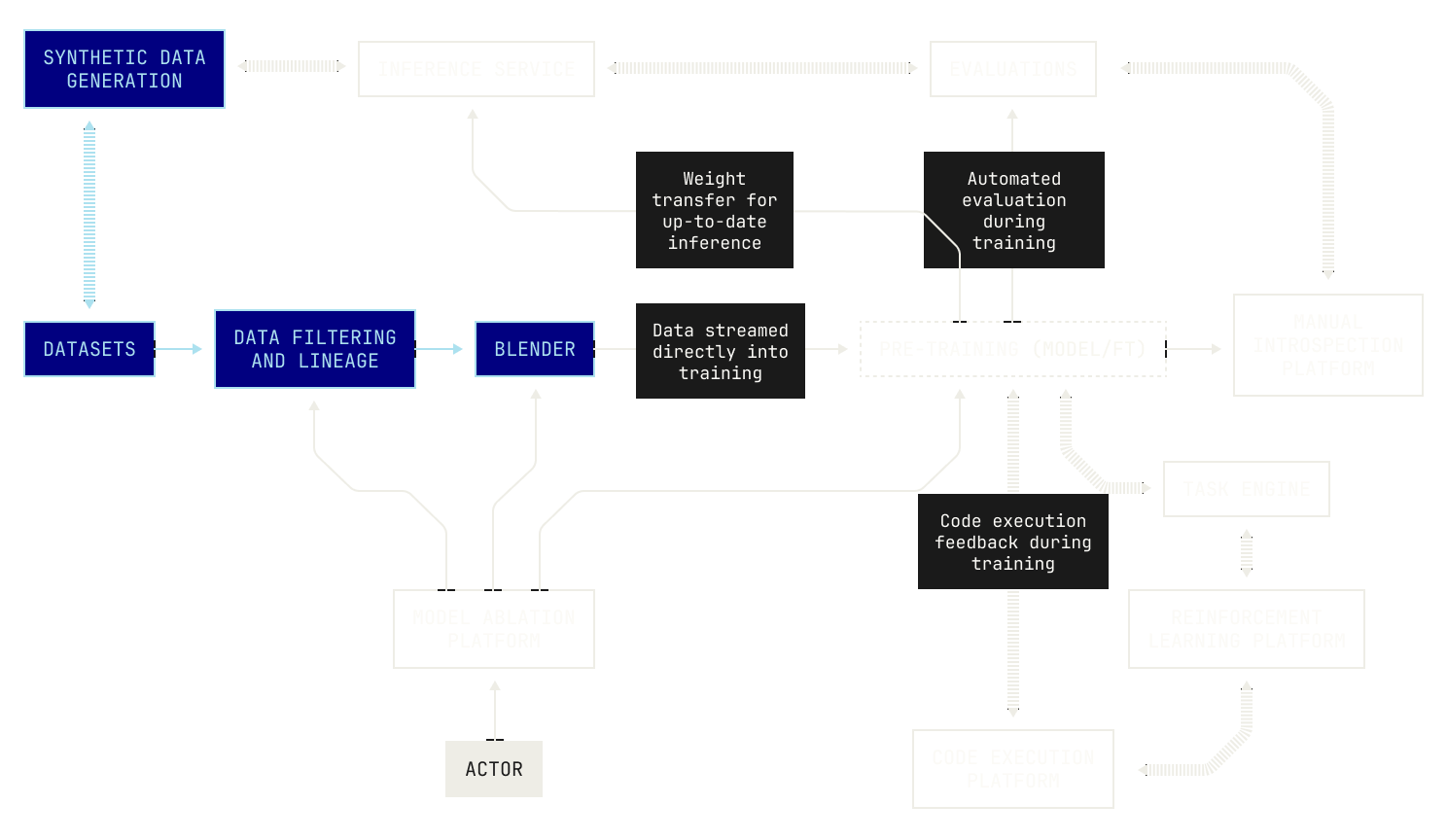
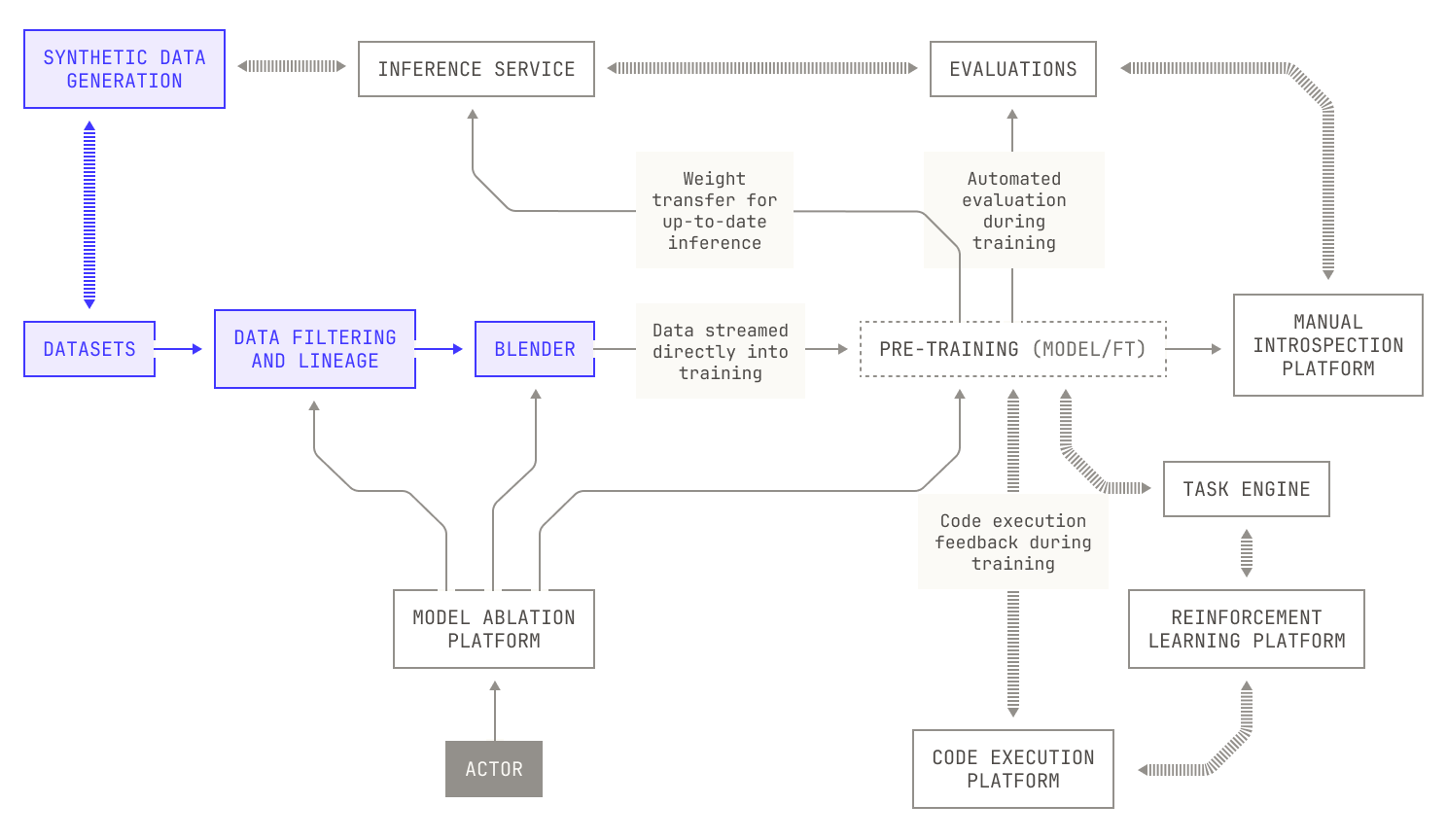
In today's post we'll dig into one of the largest parts of the Model Factory: our data pipelines. In our factory analogy, our data pipelines are where we check and process incoming raw materials before we feed them into our training machines. This covers everything from unloading raw materials into our Factory's warehouse to generating new materials synthetically to checking their quality, through to pre-processing and ultimately up to packaging into a form that suits our training machines.
Let’s get started.
Data ingestion
Before we discuss data processing, we first need to describe how we ingest data into our data lake. In practice, the data ingestion process is the most ad-hoc piece of our pipeline, as we need to handle various datasets, each with their own layout, file format, and metadata. These sources are also highly diverse, with inputs ranging from structured databases to raw files and web crawls. In order to handle this complexity, our data ingestion pipeline is both highly flexible and designed to produce data assets in a fixed form.
The first step of ingesting data is finding the right sources of data. On the one hand, there are many open-source datasets available that can be used for training, but we often find that these datasets are either too low quality or simply don’t provide enough tokens for large-scale training. Moreover, existing datasets can contain copious amounts of content that simply aren’t useful for our purposes, such as advertisements. Thus, although we do make use of open-source datasets, we also produce our own internal datasets from scratch for training our foundation models. For example, for code data, we deploy specialized pipelines that select the right data for our use cases (discussed in more detail below).
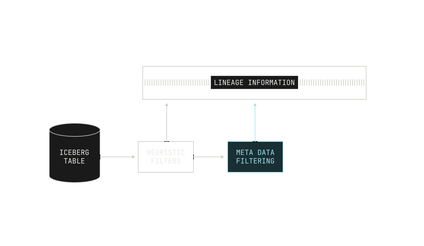
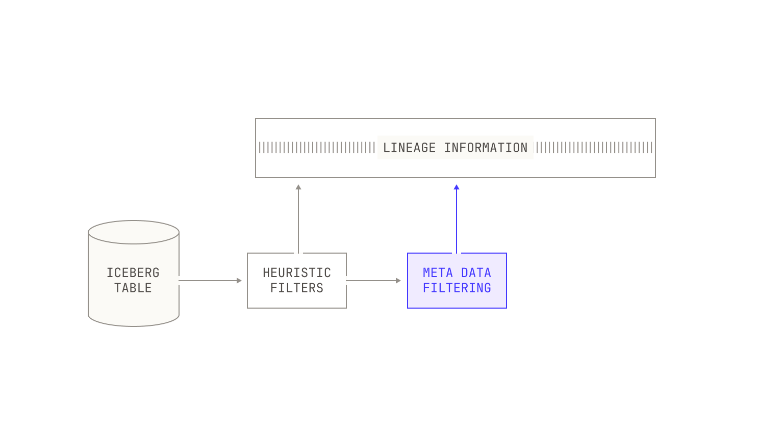
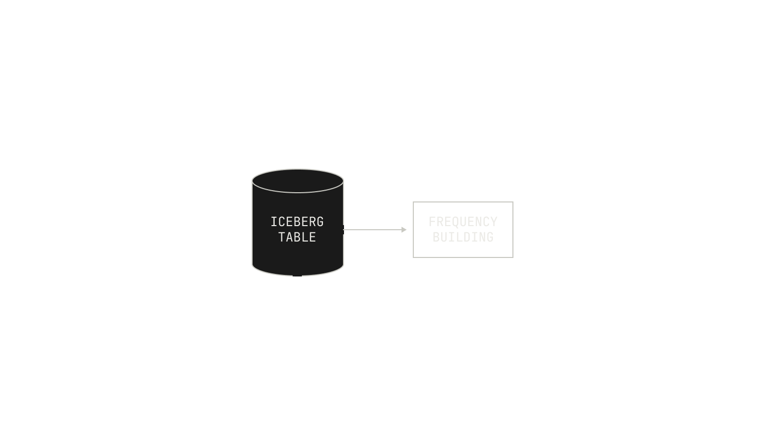
We now turn our attention to the process of ingesting data. As a recap, each dataset in our corpus is represented as a separate Apache Iceberg table.
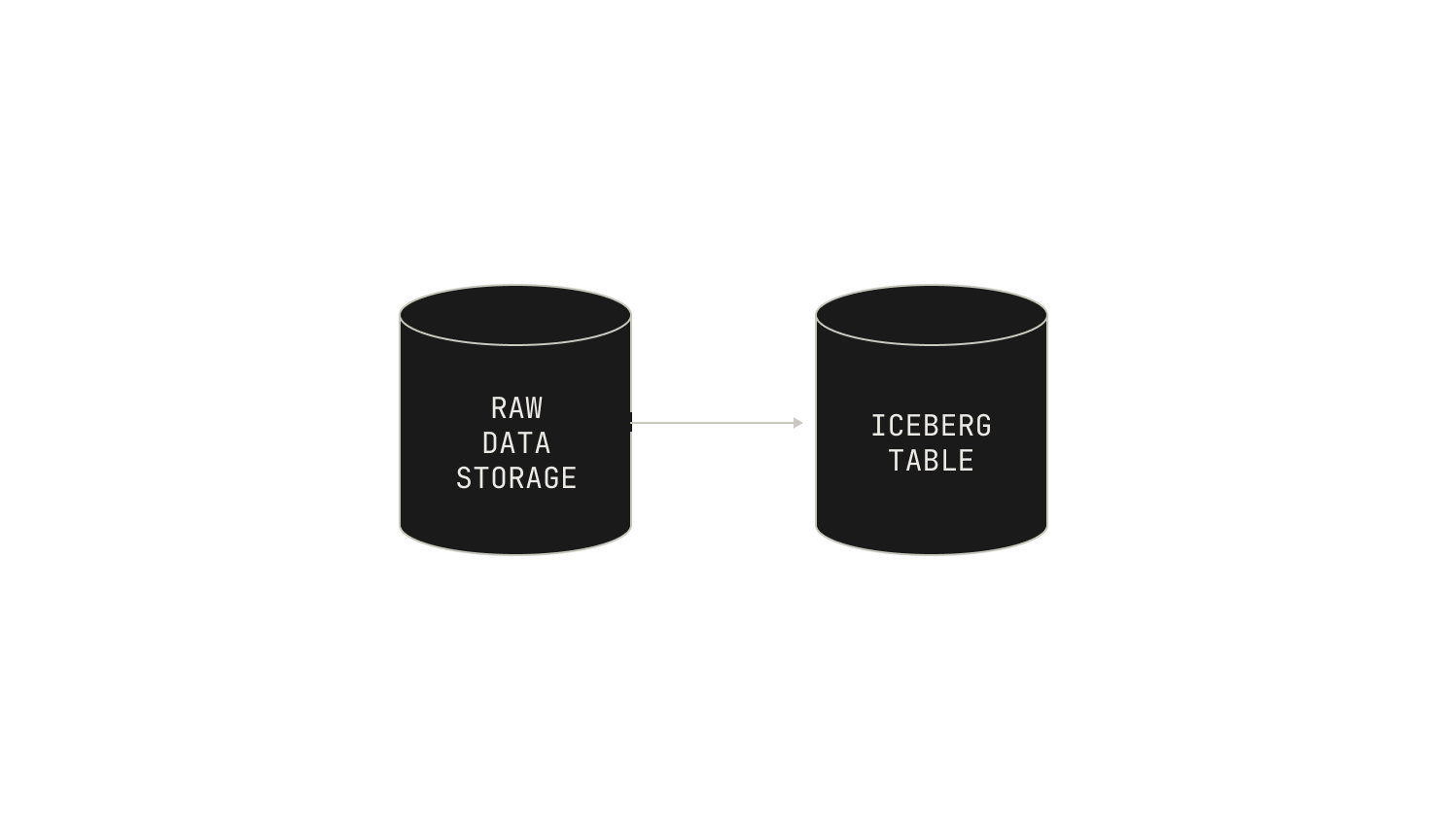
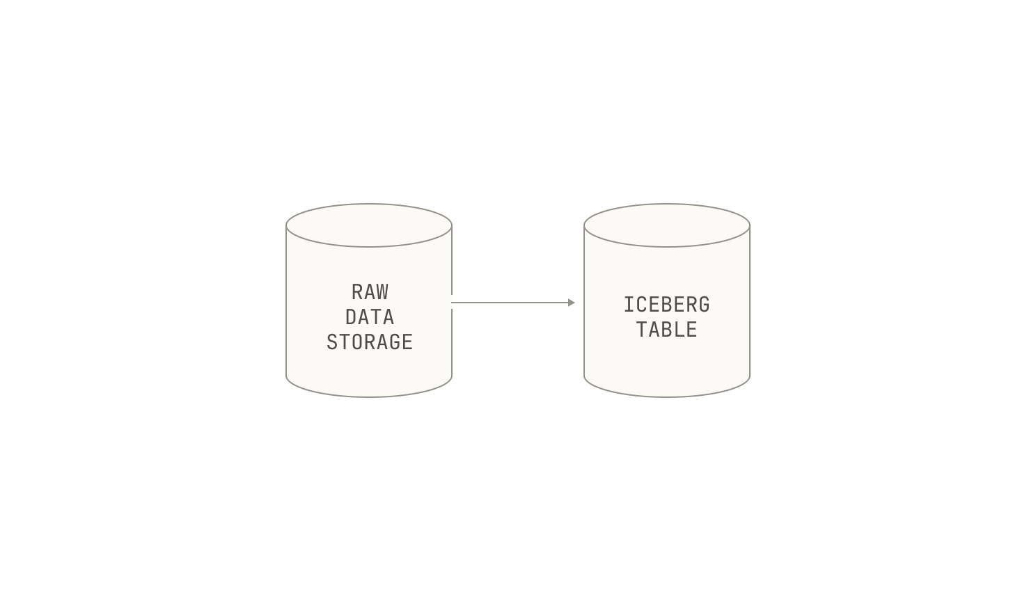
Each of these Iceberg tables are produced by a Dagster asset. Specifically, we first write a Dagster asset that defines an Iceberg table, and then we trigger an ingestion run. Remarkably, this is all it takes: Dagster’s IO engine handles the rest of the work for us.
It’s worth discussing how this process works in practice. In particular, recall that Dagster allows us to define data assets declaratively using Python decorators, with workflow orchestration handled by our CI pipeline. Notably, Dagster assets allow us to define how assets are constructed, including how the underlying data is mapped to an Iceberg table. These functions encapsulate the logic specific to each source, managing everything from connection setup to data extraction. By delegating the actual pulling process to these specialized functions, we maintain modularity and clarity in the pipeline, making it easier to extend and maintain. In other words, this approach captures all we need to handle diverse data sources; we can simply define a transformation for a particular data source and call the transformation from the asset definition.
Let's look at an example. Our Dagster assets look something like this:
@table_asset(
    group_name=”nl”,
    partitions_def=...,
    …,
)
def example_asset(context, pyspark, ingests, …) -> DataFrame:
    …
    df = …
    return df.filter(...)
The function above is just a stub, and the exact functions we use to represent and pull data depends heavily on the characteristics of the data source. For example, when dealing with natural language datasets from Hugging Face, we often encounter datasets that are stored as Parquet files. While Parquet files are highly efficient for large-scale storage and querying, integrating them into our Iceberg-based data architecture requires defining the appropriate metadata structures and transformation logic. Depending on our ingestion setup, we may be able to use these files directly, or we may need to define how to properly structure them for our downstream workflows. On the other hand, not all data arrives in this neatly packaged form, and sometimes we need to ingest data from much rawer sources. This could include unstructured files, raw logs, or even streaming inputs that require preprocessing before they can be integrated into our standard data model. Handling these cases demands custom extraction and transformation logic to ensure the data fits our downstream workflows; but, as we've seen above, doing this is not a blocker to our development.
Of course, it may also be the case that the quality of the underlying datasets is not sufficient. Indeed, we regularly encounter datasets that have been incorrectly parsed or serialized into a textual representation. In order to circumvent this problem, we perform OCR to accurately parse datasets. Notably, we deploy the OCR functionality as part of the Model Factory itself, enabling us to use all of the other tools in the Factory to investigate the efficacy of these OCR techniques relative to a preexisting baseline. For us, this integration represents an exciting frontier where computer vision and natural language processing converge to enhance dataset construction.
Code datasets present a different challenge. While code datasets do exist in the wild, they’re typically either too small or too low quality for us to use. But code repositories are typically found in only a few places on the internet, rather than across the whole internet. Thus, although existing code datasets aren’t sufficient for our use cases, we’re able to handle this problem by periodically pulling in open-source repositories (and many of their revisions) into our data pipeline. We don’t pull every open-source repository available; instead, we only pull repositories that pass our quality and licensing checks.
Combining all of these pieces together, we end up with a more complete picture of our data ingestion pipeline:
At this stage it’s worth mentioning that our data team obsesses over data quality, spending many hours inspecting datasets by hand to ensure quality. This oversight is crucial, because the work often involves nuanced decisions that defy simple automation or general rules. Our data team carefully curates the data during ingestion, ensuring that the quality is sufficient for our purposes. In addition, our engineers and researchers pay special attention to ingesting additional metadata associated with datasets; this is especially useful for our data filtration steps. In fact, one of the most useful parts of our pipeline is that we can re-run everything (with fully reproducible results) from scratch, allowing us to augment existing datasets with additional metadata.
Finally, one of the strengths of our ingestion pipeline is its ability to scale seamlessly, primarily thanks to our decision to base it on Spark. Indeed, Spark's distributed computing capabilities allow us to process massive volumes of data quickly and reliably. For instance, on baseline compute we’re able to ingest roughly 20 trillion tokens per day. The performance of this workload demonstrates both the robustness of our architecture and the efficiency of our workflows.
Synthetic data generation
While there are copious amounts of web data available to train on, these datasets only provide one piece of the puzzle when it comes to pre-training data. From a certain viewpoint, the impact of training on the web is already widely known. After all, all foundation model providers do this. But existing datasets are typically very lopsided in terms of content, and it may be impossible to find sufficiently sized datasets for certain tasks. In order to circumvent this issue, Poolside makes substantial use of synthetic data generation techniques, including at pre-training scale. Gathering this level of synthetic data is a difficult task in a non-modular workflow; however, when we came to incorporate synthetic generation into the Model Factory, we realized that we already had all of the pieces ready—we just had to put them together.
Before we continue, it’s worth pointing out that gathering synthetic data requires great care. After all, one of the reasons for generating synthetic data is to produce high-quality data of a certain kind for pre-training. We avoid using biased or low-quality synthetic data by applying judicious amounts of manual review and filtering on our synthetically produced data. We stress that this is just as difficult with non-synthetic datasets. Indeed, as all of our data pipelines in the Factory are dataset agnostic, we’re able to treat synthetic datasets in precisely the same way that we treat any other dataset; and we regularly inspect the full lineage of synthetically generated datasets.
Now let's discuss how we generate synthetic data. For the sake of example, we'll talk about how we generate code execution datasets from a set of repositories. Specifically, we produce code execution datasets by taking certain pre-defined tests and executing those tests on specified inputs, recording the output. Intuitively speaking, the goal of these datasets is to teach a model how to reason about code execution in a static context. We'll discuss the actual details of how our code execution platform works in a future installment of this series, so for now we'll just discuss the logistics of generating this data.
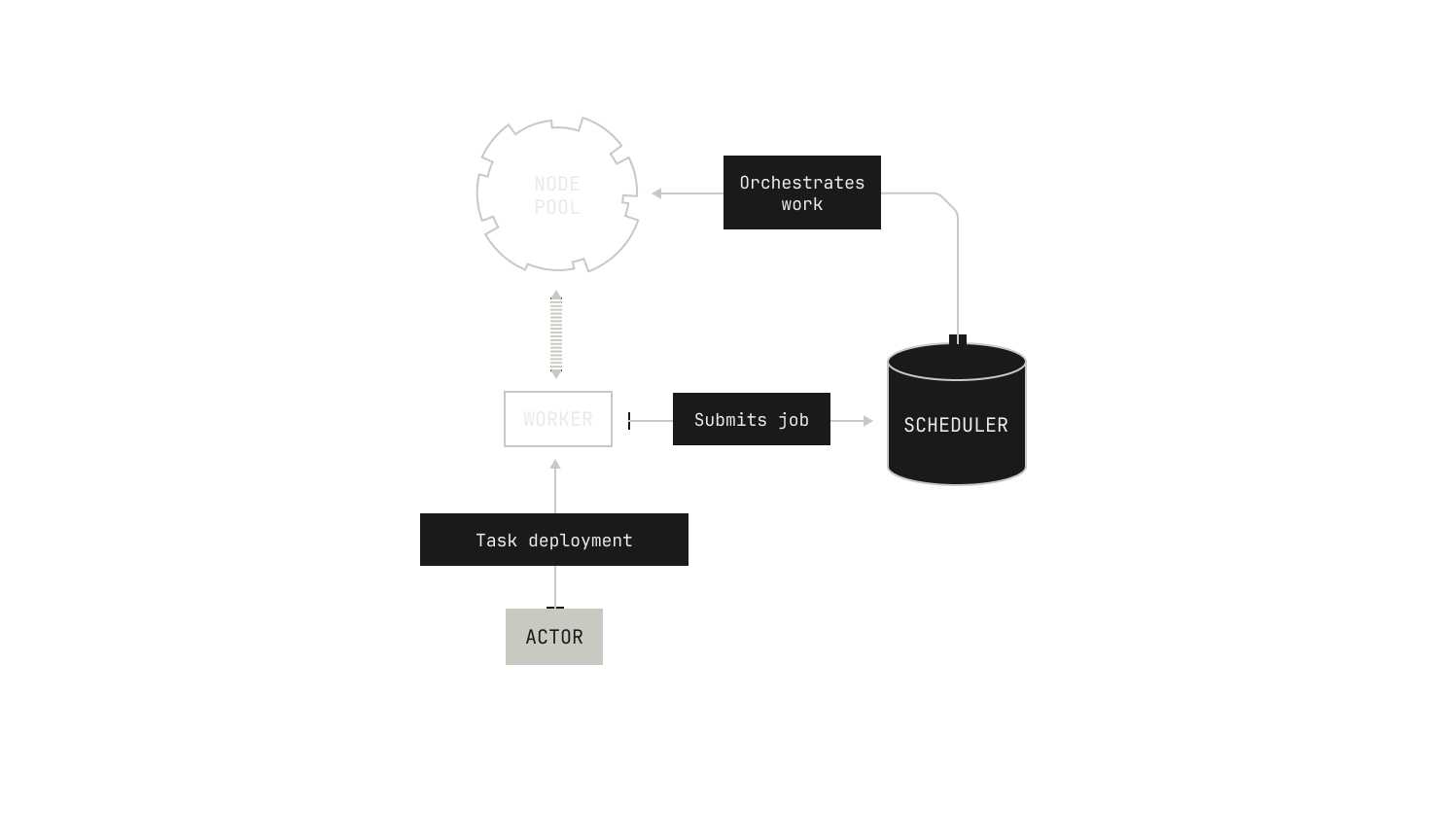
The first thing we do is deploy a worker process onto a particular node. This deployment takes some care. On the one hand, this sort of synthetic data generation is typically a low-priority task, and so we allow these tasks to be preempted from nodes in favor of more pressing compute jobs. On the other hand, synthetic data generation workloads can vary in a hard-to-predict manner, and so we typically deploy these tasks across multiple replicas behind a load balancing service. Reconciling those two separate requirements is easily handled by the Factory's orchestrator, as it has a global view of all outstanding jobs and their relative priority.
With worker deployment taken care of, we need to actually generate some data. We won’t go into too much detail here, but in this particular case, the worker can simply invoke our code execution environment with a predefined set of inputs and collect the outputs. In some other settings, we may employ an agentic setup, allowing the worker to re-interact with the code execution environment across multiple iterations. Once all of these iterations have finished, we output the resulting data into the dataset that we are building. In the case of natural language tasks, we may run a job on an existing document, such as a rephrasing job. Everything that we do during synthetic data generation is tweakable, with all steps depending on the underlying goal of the dataset. These processes typically lead to large datasets from which our models can learn during training or fine tuning.
Now, the description thus far has deliberately been structured to sound entirely manual, but in fact, it’s fully automatic. Indeed, every aspect of the pipeline is coordinated via Dagster and our orchestrator—from processing through to code execution. In fact, all we typically need to do is decide which worker to deploy, the sort of data we want to generate, and the size of the job. The Factory handles the rest. This automation removes the manual strain of generating synthetic data. We are only limited by the speed at which we can produce ideas, not by the manual workload of generating such data.
We now turn our attention to how we implement this process in practice. First, recall that all of our data is stored as Iceberg tables in a data lake. In order to create an Iceberg table for a particular dataset, we simply repeat the same steps we used for data ingestion. Namely, we create a Dagster asset that describes the underlying table, and we populate the table with data from our synthetic data generation engine. The synthetic data generation tasks themselves are triggered in the same way as any other job in the Model Factory: we simply specify the properties of the underlying job, and then Dagster handles the rest.
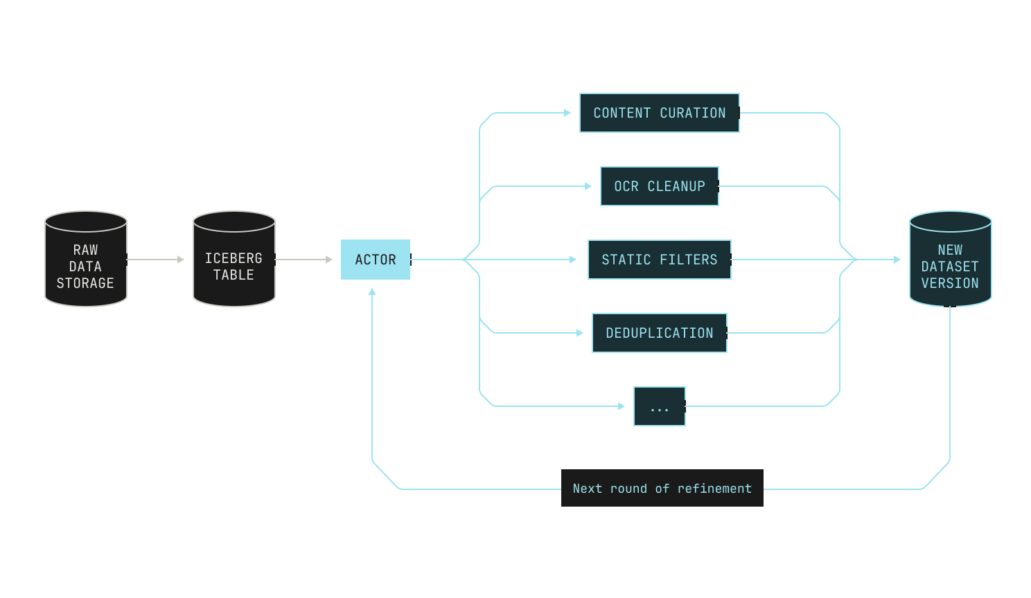
Data filtering
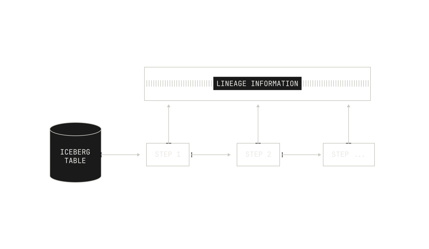
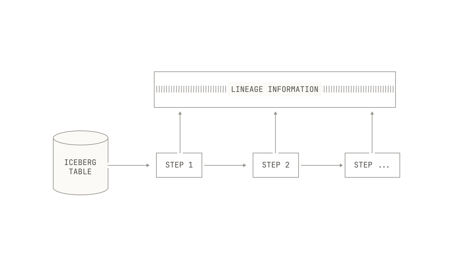
Now that we've ingested our data, we can turn our attention to the first refinement step in our pipeline: data filtering. Data filtering, as the name suggests, is the process of removing data samples from an existing dataset, with the end goal of improving the quality of the underlying data. Before we continue, we want to stress that data processing and filtering is an inherently iterative process. That is, rather than applying a single set of rules once and moving on, we cycle through multiple rounds of analysis, refinement, and reevaluation for any given dataset. Indeed, we continually apply filters and inspect the datasets to make sure everything aligns with our quality and distribution goals. While this would typically be a time-consuming task, the Model Factory dramatically accelerates the process. Indeed, the Model Factory enables us to evaluate multiple data compositions in parallel; and crucially, it allows us to trace each dataset variant back to its original source. This enables us to track how certain changes modify the quality of a given dataset.
Before continuing, let’s discuss what we’re hoping to achieve by filtering datasets. Intuitively speaking, we’re seeking to improve the quality of the data that the model sees, as this has a strong effect on downstream model performance. In order to achieve this, we need to both optimize the contents of each individual file as well as the distribution of the dataset as a whole. In the first instance, we primarily want to make sure that the language quality of the input documents is good. We look for high-quality writing, good structure, and informative content. Equally, we explicitly remove any detected content that is hateful, abusive, or profane. The second part of our filtering strategy centers around improving the quality of the dataset as a whole, and we seek to achieve two distinct goals here. First, we want to make sure that any particular dataset is appropriately diverse across content categories. Intuitively speaking, this is equivalent to removing unintentional "categorical upsampling" that may be present in certain datasets. For instance, in the past we have noticed that there is an abundance of advertisements in commonly-available web data, which disproportionately degrades the downstream performance of our models. In this vein, we broadly aim for a relatively uniform distribution of data across different document categories. Second, we seek to obtain a fairly flat distribution of document lengths; that is, we want to make sure that the lengths of the documents in our corpus follow a somewhat uniform distribution. We seek this split for two reasons: we want to make sure that our models do not only see documents of a certain length during training, as this could influence downstream model performance negatively; and we want to make sure that we have sufficient flexibility to ensure that our document packing procedure works efficiently (see the "Data Packing" section for more on this process).
In order to achieve these goals, we have built several robust pipeline steps in our Model Factory. It’s important to note that not every filtering step is deployed on every dataset, as this is not always a sensible procedure. For instance, we don’t expect most open source software to contain any advertisements, so we don’t apply advertisement-based filtration to that code. On the other hand, pure natural language data does not contain any code by definition, so applying code quality filtration here will not yield good results. In all these cases, we rely heavily on the experience of the engineers and researchers in our data team to iteratively improve our datasets; and we spend many hours manually inspecting data samples to ensure that our filtration steps do not adversely affect the quality of the underlying dataset. We do note, however, that our filtration steps are typically quite aggressive, and we sometimes end up with high-quality datasets that are only a single-digit percentage of their original size. Still, we now describe these steps in detail. For the sake of exposition, we'll focus on a cleanup of a web-based dataset that we did recently.
The first thing that we did to this dataset was apply a series of heuristic filters. These heuristic filters are designed to cheaply strip out poor quality content. Unlike the other filters in this section, these filters are rather generic, and they’re typically used to remove known bad content, such as profanity or hate speech. We also preemptively discard natural language documents that correspond to certain kinds of advertisements. We stress that these heuristic filters are not perfect, and they can miss low-quality documents.
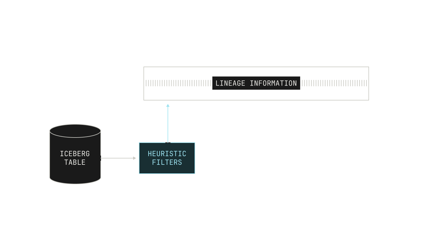
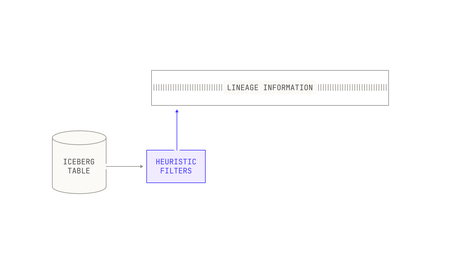
Once we've applied these lightweight filters, we typically run another filtering pass that utilises dataset-specific metadata. Specifically, documents in certain datasets—both public and private—are accompanied by additional metadata that we can use to further filter documents. We note that this filtering is typically applied on an instance-by-instance basis, and thus we don’t always apply it. For instance, if we’re interested in the baseline quality of a particular dataset, we do not typically apply metadata-based filtering. Additionally, we record the reason that any particular document was rejected from a dataset as part of the filtered asset, allowing us to inspect the quality of our filters manually. This sort of inspection is remarkably easy with the Model Factory: as every data asset is immutable and complete with its own lineage, we can always trace any document omission back to its root cause. This immutability and traceability makes improving the quality of our filters in the Model Factory incredibly straightforward.
However, lightweight filters are seldom enough to ensure that we have data of sufficiently high quality, so we need to apply some heavier filters. For instance, the data in this particular dataset was still visually skewed towards certain topics, like advertisements. This distribution clearly runs contrary to our aims of having a fairly uniform distribution of document topics. Moreover, in this particular case, we were unable to use preexisting labels for this dataset, as almost all of the documents did not have an associated label. To circumvent this issue, we applied a K-means clustering algorithm to group the documents in this dataset into roughly 15K clusters of document topics. Once this clustering was completed, we looked at the distribution of documents and noticed that there was still much more structure to the documents, and thus we repeated the K-means clustering in a more fine-grained way, this time producing around 3M fine-grained document clusters.
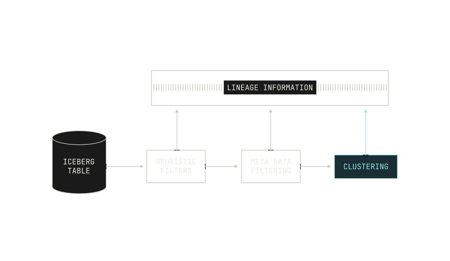
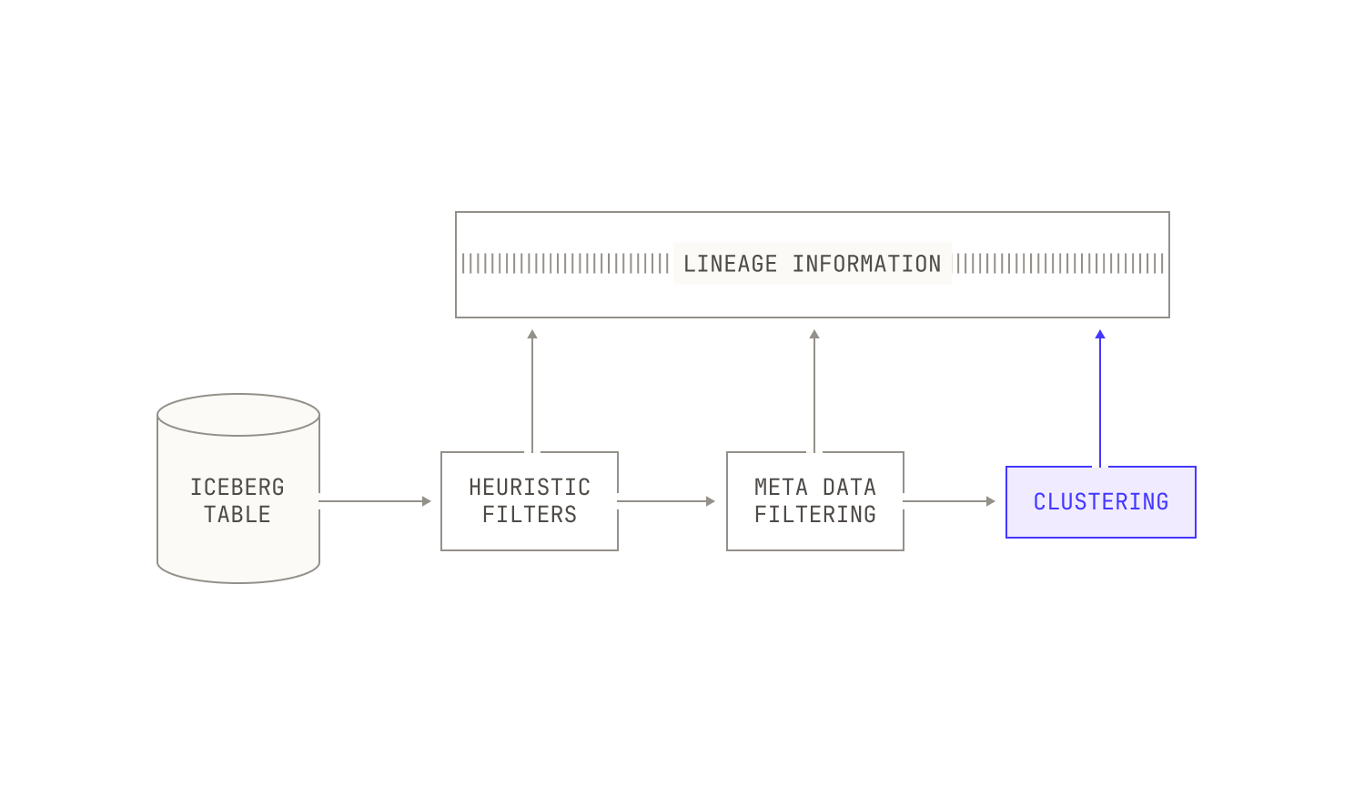
After these clusters were produced, we needed to decide which clusters to keep and which clusters to discard. In order to decide which clusters to keep, we took a proxy model that’s already been trained and continued training on each of the clusters before recording the loss. Intuitively speaking, clusters that lead to a low loss tend to be either too easy or redundant, whereas clusters that give a high loss tend to be noisy. In these settings, we simply discard clusters that lead to high loss and downsample clusters that are easy to learn. In the context of our current example, this step alone removed around 24% of the original data from our target dataset.
But just because we've discarded clusters doesn't mean that we're finished. Indeed, at this stage we noticed that the remaining dataset was still heavily skewed towards advertising data. We thus continued our cleanup by applying a simple classifier to the already filtered dataset, removing an additional 19% of the original data from the dataset. With advertisements heavily downsampled, we then decided to target improving the overall quality of the rest of the dataset. Because our heuristic filters can miss certain forms of profanity and non-English documents, we then applied tooling to detect the quality of documents. In this particular instance, we discarded documents that were either profane or contained low-quality writing. Remarkably, this led to an additional reduction of around 14%.
Before continuing, we briefly mention that this work is very much worth doing. Indeed, applying these filtering steps on our example dataset led to an improvement against the baseline on all of the pre-training benchmarks that we use, with an average relative improvement of around 5%, the largest relative improvement being as large as 150% against the baseline. This improvement is large enough that we regularly apply these steps to hundreds of datasets as part of producing our pre-training data mixes. More broadly, using data filtering (along with the other parts of our data pipelines) leads to datasets that achieve significantly better results than any currently available open source datasets across our many ablations.
Deduplication
We now turn our attention to deduplication. We'll first describe how we handle file-level fuzzy deduplication and then we'll look at repository-level fuzzy deduplication. We'll then discuss how we implement deduplication from an implementation perspective.
Before getting too far into deduplication, though, we'll first discuss why we run deduplication at all. Intuitively, deduplication improves a model's downstream performance by removing accidental data upsampling in a particular dataset; and as a result, we pay special attention to its role in our pipeline. Additionally, deduplication is the first step of the pipeline that involves interaction between multiple separate datasets—after all, we filter datasets individually—so we need to be careful to handle multiple data assets without degrading the overall dataset quality.
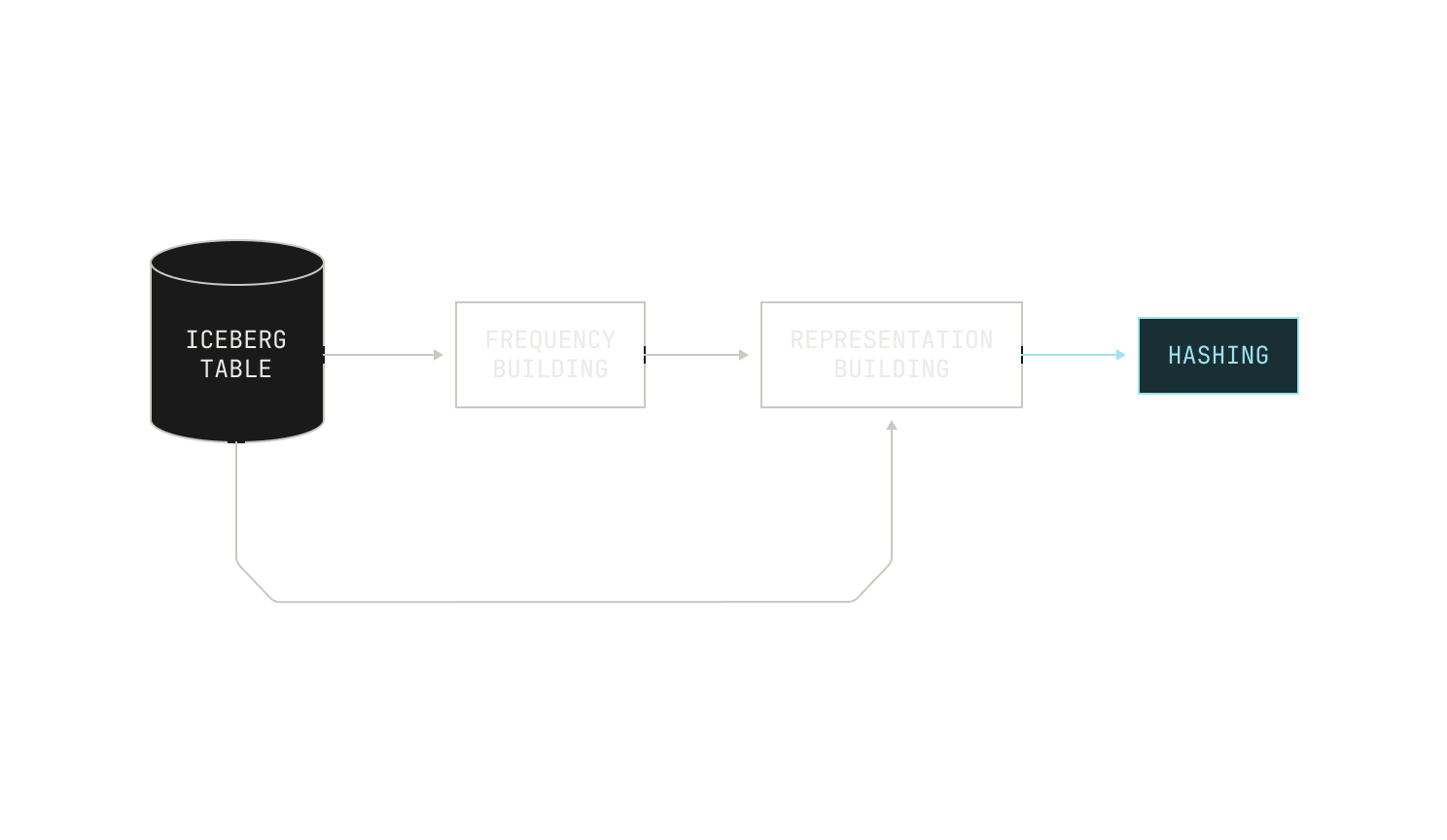
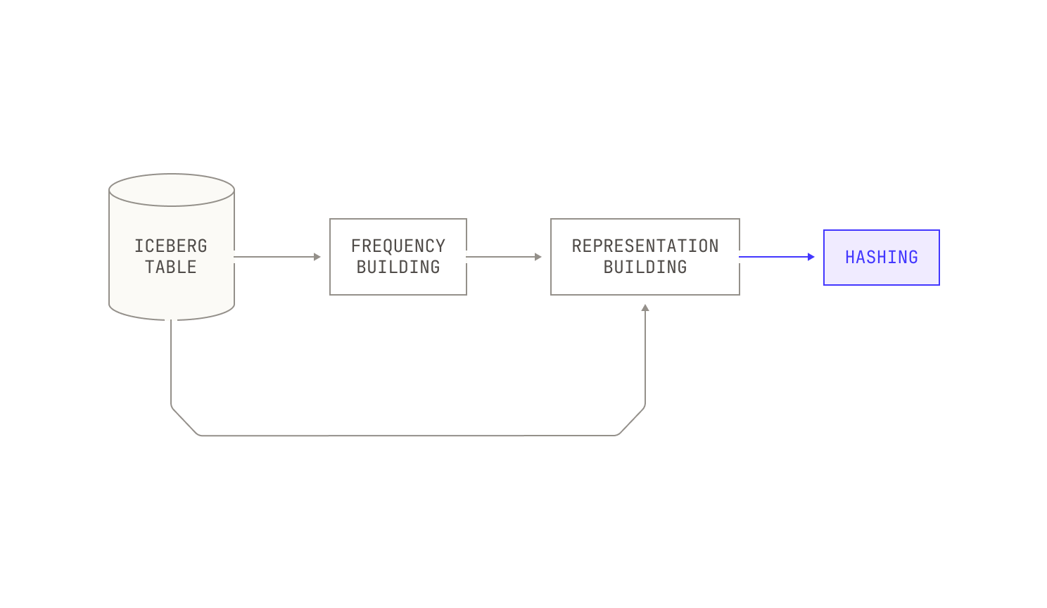
At a high-level, we apply fuzzy deduplication to our datasets by using a variant of Ioffe's Weighted MinHash scheme. We chose this approach compared to alternatives like SimHash due to its superior precision across a broad range of similarity thresholds []. This higher precision in identifying near-duplicate documents enables us to maintain the quality and diversity of our datasets more effectively. Before continuing, we recall that MinHash (and all of its variants) approximate the Jaccard similarity metric (i.e. the ratio between the intersection and union of two distinct sets). In contrast, Weighted MinHash expands on this scheme by incorporating weighting by term frequencies, producing a higher level of accuracy.
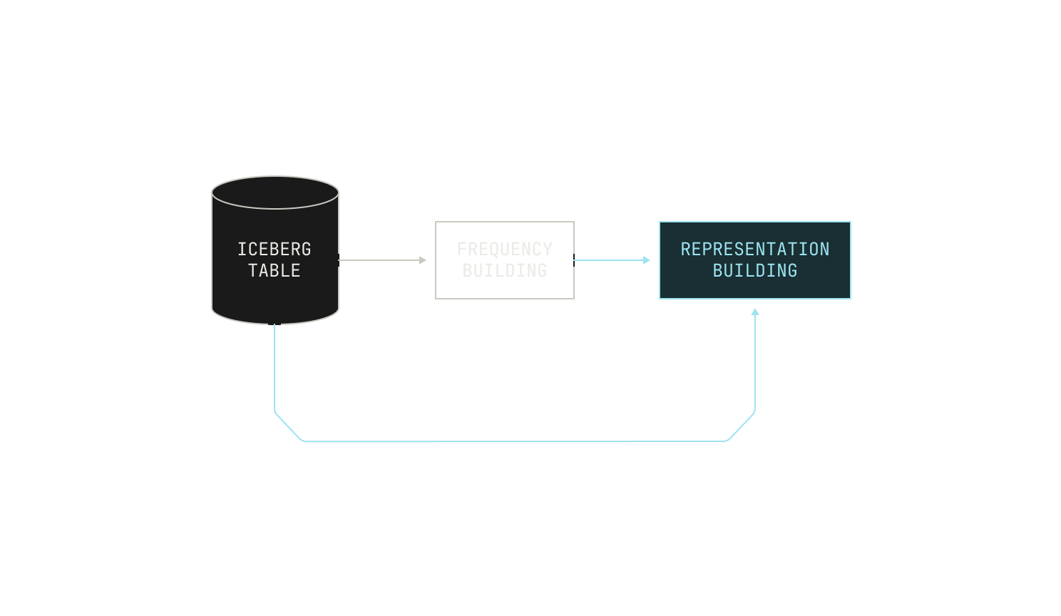
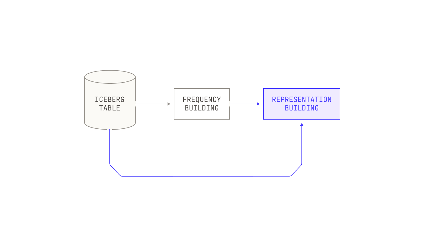
Now let’s talk about the process in more detail. Our deduplication process begins with building a comprehensive vocabulary for the entire corpus, alongside counting the frequency of each token. This step ensures that the importance of each token is properly weighted relative to its distribution across documents, setting a meaningful baseline for similarity comparisons. In the case of natural language documents, we tokenize input documents by applying a simple pre-trained tokenizer, allowing for efficient vocabulary building. On the other hand, for code documents, we apply language-specific tokenizers to ensure that certain tokens—like semi-colons—are not over represented in the final vocabulary.
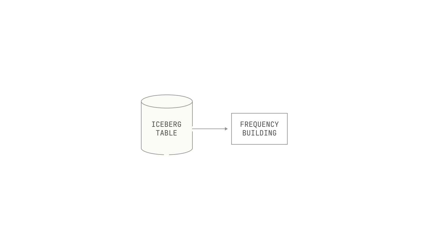
The next step in our pipeline is to use the frequency table to map each document into a new, weighted-bag-of-words representation. Each representation is accompanied by certain bits of metadata, like the document’s original identifier.
Once this representation has been built, we stream it into the actual MinHash step. Intuitively, the MinHash step accepts an input representation and produces as output a single b bit hash. We then divide this b bit hash into several bands of k bits each; each set of k bits represents a separate key in a global hash table, mapping each document to b / k separate buckets. The exact values of b and k depend on the desired similarity level, but optimal values for b and k are easy to compute for a given similarity level. Practically speaking, documents that are mapped to the same slots in the hashtable are likely to be near-duplicates under the hashing scheme.
We now need to process the buckets in our hash table. As each document is mapped to b / k separate buckets, our hash table acts as an unmaterialized graph between documents, with edges representing similarity relationships between documents. By materializing this graph, we can identify connected components of documents linked by similarity. Then, once a connected component has been found, we need to process these connected components in some way. Instead of treating each connected component as a clique (where choosing a single document would suffice), we approach the deduplication problem by solving the search Vertex Cover problem on the connected components. This choice is motivated by the fact that similarity edges are not strictly transitive, and simply picking one document risks losing important content. The Vertex Cover solution selects a subset of documents that collectively "cover" all similarity edges, which better preserves the variety within each component. Practically, we apply a straightforward greedy heuristic to approximate the Vertex Cover, which performs comparably to exact solvers in most cases.
Finally, we typically run the deduplication pipeline multiple times at varying similarity thresholds before selecting the final dataset for training. This multi-stage process balances dataset size against output quality: higher similarity thresholds reduce duplicates more aggressively but risk losing diversity, while lower thresholds preserve more data but may retain unwanted redundancy. Through careful tuning of these parameters, we ensure that the resulting dataset maintains both quality and efficiency for downstream training tasks.
Now that we’ve discussed how we’ve applied fuzzy deduplication to documents, we can address how we handle repository-level deduplication. We follow the exact same procedure as in the file case until we've produced the set of connected components. Once we've produced the set of connected components, we simply map the nodes in the graph back to their original repository, combining all of the nodes that correspond to the same repository. But in contrast to file-level deduplication, we have two additional concerns to handle. First, we still need to handle the fact that around 40% of repositories are grouped into a single large component. To handle this, we additionally apply a labelling mechanism, grouping repositories by their broad topics. Whilst this means that components no longer correspond to exact duplicates, we can more easily strip out repositories that do not correspond to what we’re looking for. On the other hand, we also want to make sure that we are retaining repositories that are known to be good; after all, we do not want to keep forks of projects if we can keep the original version instead. This simply requires us to modify our Vertex Cover algorithm slightly to take additional metadata into account, allowing us to keep high-quality repositories in the output of our repository-level deduplication.
Before wrapping up, it is worth discussing how our deduplication pipeline has evolved over time, as it highlights how the Model Factory has helped us scale our efficiency in practice. In the beginning—that is, long before the Model Factory existed—we implemented deduplication as a single end-to-end program that ran on a u-24tb1.112xlarge EC2 instance, furnished with 24TB of system memory. Predictably, it did not take long for us to feel the strain of using this approach, so we re-implemented deduplication as a series of pipelines that each operated independently. Notably, this particular approach suffered from several bottlenecks: there were several sub-steps that were limited to a single machine, which massively increased the amount of time needed to run deduplication. Worst of all, running deduplication in this way required a huge amount of manual interaction; jobs needed to be manually launched, and failing jobs needed to be manually resolved. This had a curious knock-on effect; we found ourselves trying to avoid exercising the full deduplication pipeline for small datasets, as the manual workload was simply too high. This knock-on effect gave rise to all manner of hacks—some of which turned out to actually be very insightful; but this example highlights that our deduplication pipeline simply wasn't where it needed to be for Factory-level usage.
When we came to build the Model Factory, implementing a robust and easy to use form of deduplication was top of our wishlist. To achieve this, we modelled deduplication in the same way as the rest of our data pipeline: we still treat each step of deduplication as a separate program, but each separate program now heavily utilises Spark, enabling easier scalability. Of course, not every step is trivially parallelizable, and we had to pull some tricks out of our algorithmic toolkit—like massively parallel connected component algorithms— to eliminate any single node steps. Moreover, we orchestrate deduplication using Dagster, which enables us to easily manifest intermediate results as data assets. This decision, it turns out, was remarkably useful. Materialising intermediate results as Iceberg tables enables us to easily track lineage and identify the impact of each processing step. Better still, by producing intermediate steps in this way, we can more easily recover from failures or disruptions in individual steps.
The improvement from the Model Factory version of deduplication relative to the older version cannot be overstated. Before, deduplication was a heavyweight process to run that required near-constant babysitting and management to handle correctly; now, it is just another "click of the button" data workflow in our wheelhouse. Notably, making deduplication just another piece of the Model Factory pipeline opened up its usage for all sorts of unexpected use cases, and we now deploy full deduplication on all manner of datasets when we simply didn't before.
Dependency sorting
We now turn our attention to how we package documents in a form that makes them useful for training. However, before we dig into how we actually pack documents, we first need to talk about how we ensure that our model sees documents in an order that makes for efficient training. For the sake of this section, we'll focus only on code documents, as the considerations for natural language are much less onerous.
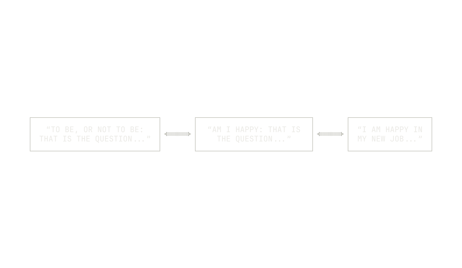
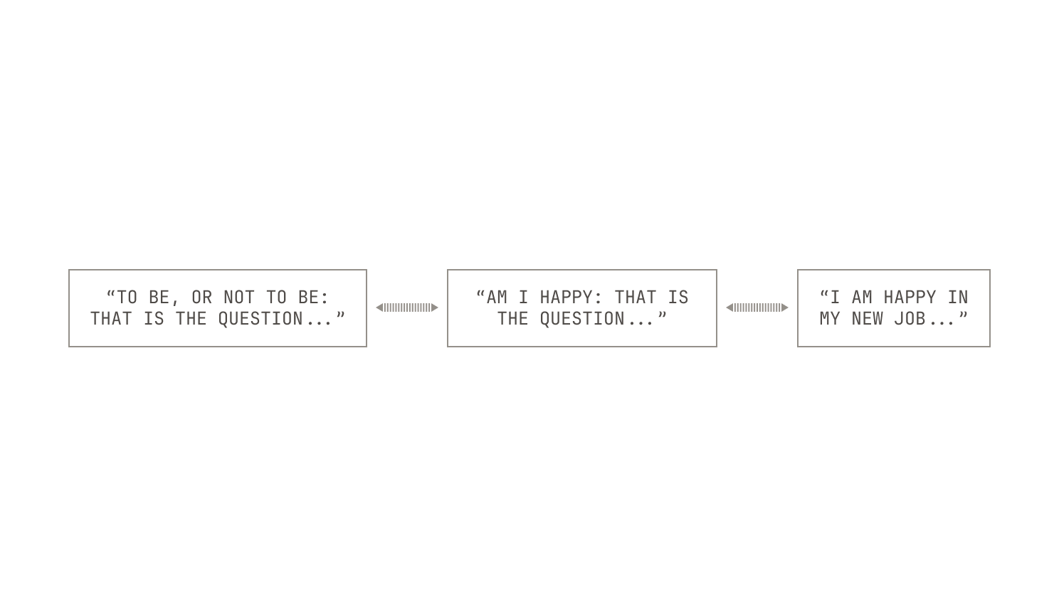
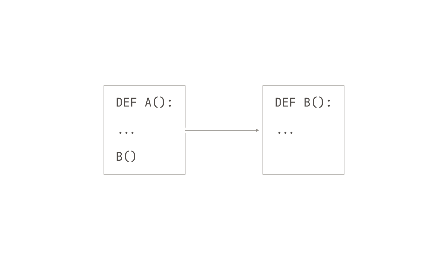
Foundation models that are trained using next token prediction rely on context to perform properly. Indeed, this is somewhat obvious in the context of natural language. We could hardly expect a model to learn if we arbitrarily swapped the ordering of certain paragraphs. However, when we supply code documents to the model, we also need to ensure that the model sees all of the relevant context ahead of time. To see that this matters, consider the following C program:
#include<string.h>

void our_memcpy(void* dst, void* src, size_t nbytes) {
     memcpy(a, b, nbytes);
}
It is clear that including the contents of this program without first including string.h is unlikely to provide the model with enough information to accurately predict future tokens. In other words, we need to ensure that we provide code in dependency order to the model during training. We refer to our technique for handling this problem as dependency sorting (or Depsort for short). In algorithmic terms, this process corresponds to computing a topological sort of a graph, where the goal is to arrange nodes (in this case, files) in an order such that each node appears before any nodes that depend on it. This process isn’t as straightforward as it might sound. While it’s well known that DAGs always have at least one topological ordering, it’s not necessarily the case that our input graphs are acyclic. In other words, we cannot assume that a strict topological sort is well-defined for our input graphs. To address this problem, we apply what we refer to as a best-effort topological sort; that is, we instead compute an approximation of a topological sort that preserves as much dependency information as possible without requiring the absence of cycles.
Let's suppose we want to apply Depsort to a project's repository. The first thing we need to do is build a dependency graph between all the files in the project. However, the process of constructing this dependency graph is non-trivial. Instead of relying on heuristic approaches such as grep or other text-based search tools, which can easily miss certain relationships— especially in languages that permit complex or cyclic inter-file references—we use a more rigorous approach. Specifically, we note the code files themselves contain all of the information that we need to extract dependency information in the form of symbol-level information, such as functions and classes. In fact, we’ve already implicitly used this information in our previous two examples. Thus, we first extract the symbol-level information from the project's abstract syntax tree and then detect which files use which symbols. This approach is equivalent to building a dependency graph; for instance, if file X defines a particular function foo() and file Y calls foo, then clearly file X is a dependency of file Y.
After we've extracted these file dependencies, we execute a variant of the classical topological sorting algorithm on the dependency graph. Our variant, in particular, works by running a depth-first search on the dependency graph. This approach implicitly treats the dependency graph as a tree, and thus any and all cycles are broken in arbitrary places during traversal. This, of course, is purely heuristic, and we are not guaranteed to produce the "best" possible topological sort. Yet, in practice, this arbitrary breaking does not appear to negatively influence model quality.
The approach described above is, of course, just one possible implementation. In some programming languages, additional information about project structure is available—most notably, in the form of packages. When package-level metadata is accessible, we take advantage of it by performing the topological sort at two levels: first across packages to resolve high-level dependencies; and then within each package, to sort individual files. This extra level of sorting gets us closer to the "best" possible topological sort without adding much extra complexity to the Model Factory.
Data packing
Now that we've established a dependency relationship between our coding documents, the next step is to organize and package these documents in a form suitable for training. This step is crucial for optimizing how we present data to the model, especially when working with limited context windows and massive datasets.
This packaging process is primarily aimed at improving the efficiency of our foundation model training. Rather than padding each document to fill the entire context window—an approach that wastes space and computational resources—we instead pack multiple documents together into a single context window, maximizing the amount of available tokens per training example. This approach comes with some complexity, as we now need to ensure that these documents do not interfere with each other during training; however, handling this is relatively straightforward, and we'll discuss this in our post on our training pipelines.
For the sake of exposition, we'll first focus on packing code documents inside a single repository. First, we sort all tokenized documents using specific metadata, such as their output order from running the topological sort described in the previous section. For documents that exceed the target context size, we segment them into smaller chunks to ensure that each piece can fit within the packing constraints. Once this pre-processing has finished, we now need to actually pack the documents. In the most basic case, we map documents to packed documents by producing a "packing plan," that is, a mapping that translates documents (or chunks of documents) into packed documents. We typically produce this plan by using the well-known best-fit packing algorithm. Before continuing, it is worth discussing why we use best-fit over other approaches. We originally used a next-fit scheme, which simply added documents one after another until a context window filled up. However, this resulted in about 15% unused space due to inefficient packing. Best-fit, by contrast, simply provides a much tighter packing, often nearing 100% utilization of the context window. Once the packing plan is established, we generate the final packed documents by concatenating the input documents in the order dictated by their associated metadata and packing keys.
The previously-described approach works well for small code repositories. However, using a single, global plan doesn't scale particularly well; producing a packing plan may only be a linear time operation, but it is tricky to scale across a cluster of machines. To fix this issue, we use a hybrid approach and define multiple sub plans for packing. In particular, we employ a pre-hashing step to split up our repositories. Namely, we first map each repository to one of several thousand buckets, and then we further sub-divide these buckets into chunks of a few thousand documents each. We then apply the packing process independently to each chunk of documents, enabling us to scale this process efficiently across a whole cluster of machines.
The approach described thus far only applies to code repositories and documents. However, our procedure for natural language documents is broadly the same; we simply treat each individual text document as its own standalone repository, and repeat the same procedure as described above. This approach ensures that document-level integrity is preserved— after all, we do not package repositories across buckets—and we’re able to reuse our existing pipelines for document packing.
Data blending
Lastly, let’s discuss how we produce and manage data blends for training. In order to describe this process, we need to first introduce our internal platform for producing data blends, aptly called Blender.
Before we dig into Blender, it’s worth reiterating what we are attempting to achieve. In traditional foundation model training, data blending is tightly coupled with data distribution: we first need to produce a blend, and then ensure that the blend is distributed to the appropriate nodes. In the past, we would have done this manually: we would have fully materialized several datasets, then we would have manually computed an appropriate blend, and then we would have distributed the dataset across the nodes. This approach, whilst workable, seriously lacks flexibility. We clearly need to know the number of nodes ahead of time. Otherwise, we wouldn't know where we need to place the blended dataset. Moreover, we also need to fully materialize the datasets and decide on a data blend before we distribute the datasets; this makes it difficult to adjust for mistakes. It’s also clear that this approach means we can’t easily handle live data sources; we would need to capture a portion of a live source, distribute it, and then repeat this process as the live source evolves. This approach clearly won’t scale across multiple live sources and multiple data mixtures. To solve this problem, we built Blender, our internal platform for configuring and fetching blends. As the name suggests, Blender provides utilities for producing data blends from multiple sources, including live sources. In practice, Blender acts as a data streaming service that allows us to easily fetch from a wide variety of Iceberg tables according to a pre-defined set of criteria. Notably, these tables are pre-tokenized and packed according to the techniques in the previous section, decoupling these details from the data streaming and blending.
Under the hood, Blender provides two gRPC services. First, Blender provides an API call that produces a configuration, called a BlendConfig, for a particular data blend. Each BlendConfig is an immutable object, and updates to an already existing BlendConfig simply produce a new BlendConfig. BlendConfigs are composed of several data sources, called BlendSources, and each BlendSource contains precisely the information needed to read from a particular Iceberg data table or table snapshot. Notably, each BlendSource contains the number of rows of the table that should be read at once, as well as if the data source is "live" or if it should be over-sampled. We refer to the number of rows in the data source that should be read as the "weight" of the source.
Once we've defined a BlendConfig, we can fetch data by calling the second gRPC service provided by Blender—the one that actually provides data. Each time the data query service is called, Blender iterates through the tables specified in the BlendConfig and returns a subset of the rows from each table. As previously mentioned, the precise number of rows returned from each table is specified by the weight in each table's BlendSource. In situations where not enough data is available for a particular request, such as when reading from live tables, Blender simply blocks until enough data is available. In any case, once Blender has gathered the data for the request, the results are streamed back to the calling node for use during training. Additionally, each response from this service also contains the current offset from the front of the blend, enabling us to either re-fetch previous data in the case of investigating loss spikes, or to fetch fresh data for subsequent training steps.
Blender is our internal platform for configuring and fetching blends from our training datasets. As a reminder, we represent our training datasets as Iceberg tables that are tokenized and packed using the techniques from the previous sections. Blender itself is structured as two gRPC services: one that allows us to configure data, and one that allows us to fetch the data from various training dataset tables.
Finally, as you’ve seen, Blender makes producing complicated data mixes remarkably easy; we simply need to specify the correct BlendConfig and BlendSources. This is a drastic change from what we had before. Previously, we had to manually pre-distribute data, decide on the mix ahead of time, and pre-reserve nodes. Whereas before we would spend a lot of time building blends, we can now simply specify what we need and Blender handles it for us. This ease of use turns data blending into just another piece of our Factory, and we can now easily experiment with multiple different data blends in places where we just couldn't before. This is especially useful in the case of reinforcement learning workflows; but for more details on that, you’ll have to wait for a future installment!
Thank you
We hope you enjoyed this tour of our data pipelines and workflows. Join us again next time for a discussion of our large-scale pre-training codebase, Titan.
Acknowledgments
We would like to thank Poolside’s data and applied research engineering teams for their thoughtful comments and insights on this post.
Interested in building machines for Poolside's Model Factory? We'd love to hear from you.
→ View open roles