TL;DR: We wrap up our series on the Model Factory with an explanation of how we use it to conduct post-training at scale. Specifically, we begin by discussing two of the post-training techniques that we use at poolside: supervised fine tuning (SFT) and reinforcement learning (RL). We discuss how the Model Factory supports orchestrating large-scale post-training workloads, using SFT and RL workloads as examples. We then conclude by introducing two tools that we’ve built for post-training at poolside: a dataset viewer, called Podium, and GPU<>GPU weight transfer.

Introduction

In the previous posts in this series, we’ve discussed almost every aspect of the Model Factory. We’ve built everything that we need to process massive datasets, quickly train excellent foundation models, teach models to code, evaluate specific capabilities, and serve inference at scale. But there’s still more to do to produce foundation models that demonstrate useful abilities in real-world environments. Moreover, we want to produce models that exhibit capabilities beyond those that can be granted by traditional pre-training alone. In order to achieve these aims, we’ll need to employ some additional techniques.

In this post, we’ll discuss how we conduct post-training on our models at poolside. In particular, we’ll consider two aspects of our post-training pipelines, namely supervised fine tuning (SFT) and reinforcement learning (RL). We’ll start by explaining why we conduct post-training on models at all, introducing SFT and RL along the way. We’ll then discuss how we’ve already introduced almost all the pieces needed to orchestrate and deploy post-training workloads, using SFT and RL workloads as examples. Lastly, we’ll conclude by discussing two systems that we’ve built for post-training workloads, namely a dataset viewer and GPU<>GPU weight transfer.

Before we get started, it’s important to remember that this post in particular shouldn’t be consumed in isolation. In fact, every post in the Model Factory series has led up to this one because post-training reuses components that we’ve already introduced earlier in the series. This is intentional: reusable components and large-scale orchestration are two of the main reasons why the Model Factory is such a powerful tool for building best-in-class foundation models. Here, we’ll focus on new features that we’ve added to the Model Factory to enable post-training workloads, as well as how we orchestrate our existing components to support running these workloads at scale.

Let's get started.

Why do we carry out post-training?

Let’s start with a brief recap of foundation model training. As we mentioned in the first post of this series, typical foundation model training starts with building an initial dataset on which to train our model. We then use that dataset to conduct an intensive training period, known as pre-training, which produces a trained base model.

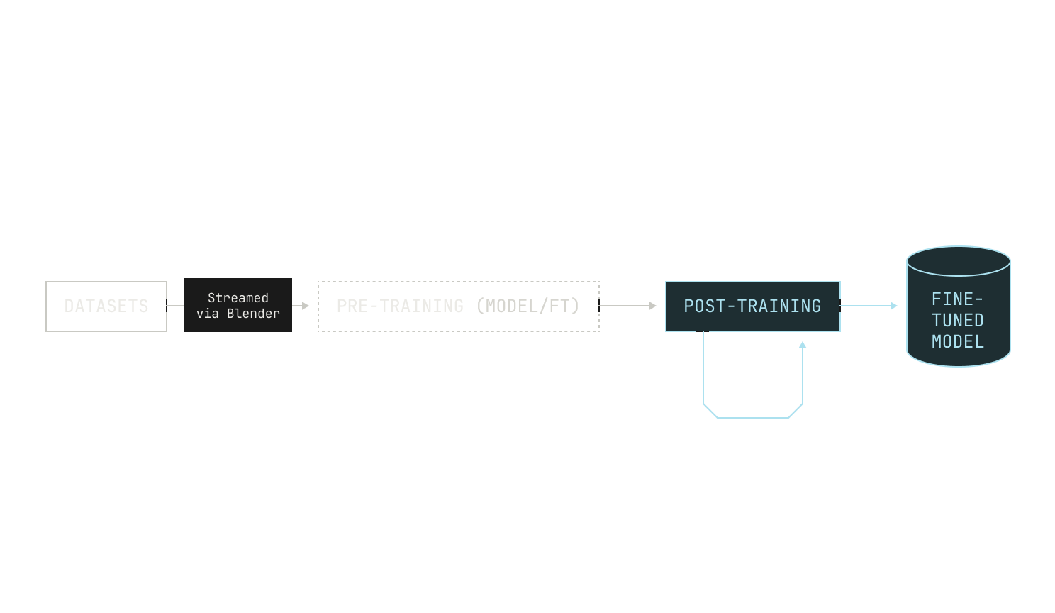
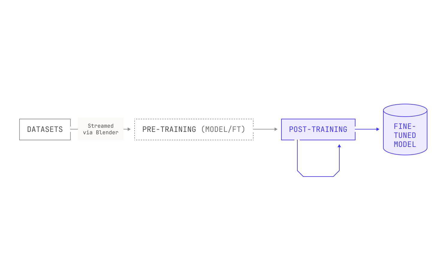
While base models are knowledgeable, they’re not normally good at problem solving. As a result, it’s common to carry out some extra steps after pre-training, known as post-training. The goal of post-training is to produce a model with specialized capabilities, like instruction following or proficiency at certain tasks. Essentially, post-training can be seen as the process that upgrades a basic text completion model to an assistant that can handle conversations, use tools, think explicitly, and solve various problems. As we seek multiple behaviors and capabilities from our models, post-training may be conducted over multiple rounds, leading to the following picture:

It’s important to note that post-training shouldn’t be viewed as a mere add-on to pre-training. In fact, post-training is essential to produce models that are usable and intelligent in practice. As a concrete example, we’ll consider poolside’s primary use case: producing models that excel at software development. While base models are typically knowledgeable about language syntax and math, there’s a huge gap between basic knowledge and being a good software engineer. This is even true in humans: software engineers require a great deal of operational knowledge and expertise to be effective. Models are no different, and there is a big difference between a good base model and a model that can act as an effective coding agent inside a real-world environment. As a result, we invest a considerable amount of compute and effort into our post-training pipelines, ensuring that we build models that are actually useful in practice.

Let's consider two distinct forms of post-training: namely, supervised fine tuning (SFT) and reinforcement learning (RL). Before we get into how we build these workloads in the Model Factory, we’ll briefly highlight how we use both SFT and RL at poolside.

On the one hand, we typically use SFT to coax a model into exhibiting predictable behavior, like producing structured outputs or demonstrating a particular “personality.” We also use SFT to provide a “warm start” for RL workloads. In practice, we follow a standard SFT workflow: we’ll build an SFT dataset, continue training on a pre-trained checkpoint, and then store the resulting checkpoint. And, similar to our pre-training workloads, we regularly run evaluations during our SFT experiments, allowing us to understand how our models change during SFT experiments. We’ll discuss the technicalities of running SFT workflows in the next section, but it’s worth keeping in mind that the real difficulty is generating high-quality datasets, and almost everything else that we need for SFT is already implemented in the Model Factory. In fact, our engineers and researchers that work on SFT spend a great deal of time manually inspecting and iterating on SFT datasets to ensure their quality. We’ll discuss a tool that we built to make this process easier (Podium) in an upcoming section.

Meanwhile, we typically deploy RL algorithms when we’re trying to teach our models to exhibit longer-term reasoning and intelligence. For example, we use our Reinforcement Learning via Code Execution Feedback (RLCEF) technique to teach models to reason and understand various software-engineering-related problems. Importantly, our RL workloads lean heavily on the other infrastructure in the Model Factory, as they require both a great deal of orchestration and compute to run successfully. As an example, our RLCEF technique requires us to ingest and process a large number of tasks, execute code to solve those tasks, and adjust to feedback. Not only does this process require a large amount of general purpose compute, but it also requires near constant access to a high-performance inference service.

It’s worth noting that we run RL in large-scale, asynchronous settings. In practice, this means that we run acting and training on distinct nodes, leading us into off-policy RL workloads. This is primarily for scalability reasons (i.e. we need to run RL workloads asynchronously for us to scale efficiently). This mandates that we carefully synchronize weights between nodes that run training and nodes that run acting. We’ll discuss a high-level overview of a technique we use for this later in this post, called GPU<>GPU weight transfer.

The Factory already enables post-training

Now, let's see what we need to run post-training workloads. It's very simple:

sft_asset = model_asset(model_name=”sft”, job_config={...}, ...)

That's it. All we need is an appropriate configuration file, and the Factory handles the rest.

This might seem like a very brief description, but that’s the point. It's our contention, at this stage in our series on the Model Factory, that the particularities of the workloads are almost irrelevant. In our view, the main advantage of the Model Factory is that it enables automated, end-to-end orchestration of workloads across multiple scales. The Model Factory contains many useful components, yes, but the components are just pieces of the broader puzzle. Instead, the major benefit of the Model Factory is that it provides mechanisms for automatically scheduling and orchestrating arbitrarily complicated systems in a fault-tolerant and reproducible manner. Without these automation mechanisms, the Model Factory would be a far less useful system for us, even if we retained every other component. Put differently, the components of the Model Factory are worth more than the sum of their parts because of the automation we’ve implemented, and not the other way around. In fact, our post-training workloads are almost entirely enabled by Factory components that we've described previously; there are only a few extras that we’ve needed to build to make things work. Put differently, because of the Model Factory’s structure, we get the ability to conduct large-scale post-training workloads at scale almost for free. Of course, we sometimes need to build new components for certain tasks, or for certain quality-of-life improvements, but ultimately these components are typically beneficial additions, not prerequisites.

Before we get into the details of each workload, it’s worth further describing how we structure experiments in the Model Factory. Although we’ve mentioned them in earlier posts in this series, all of our experiments are based on configuration files. These configuration files can be produced in one of two ways: as manually built, raw Markdown files, or programmatically from inside the Model Factory. Notably, these Markdown files allow us to specify details for every piece of an experiment. On the one hand, they allow us to specify all manner of arguments and details, from learning rates to the number of GPUs. These form the basis of our experimental workloads, and their light structure makes it very easy to launch new experiments without needing to build a new and complicated configuration file. On the other hand, we also specify the precise images that should be used for any particular experiment in the configuration. This means that all of our experiments are perfectly reproducible and repeatable—indeed, other than in the case of hardware failures, we should get an exact match for any runs launched from the same configuration. And because we launch based on exact versions, our experiments tend to only require minimal changes when other aspects of the broader Model Factory change. When we add this to our broader systems in Dagster, we end up with something quite remarkable: a fully reproducible log book of every experiment that we run at poolside. In our experience, using Dagster in this way has massive communication benefits. For instance, it's much easier to share in-progress experiments in Dagster than it was before we'd built the Model Factory. And because everyone can see the experiments, there are no silos: everyone in the team can see and ask about your experiments. This focus on collaboration also means that we've ended up prioritizing re-usable code, leading to fewer one-off scripts and pipelines. In our opinion, this is one of the best things about the Model Factory: when everyone prioritizes building strong, reusable components, the benefits compound, and ultimately building new things properly becomes more convenient than hacking things together.

SFT in the Model Factory

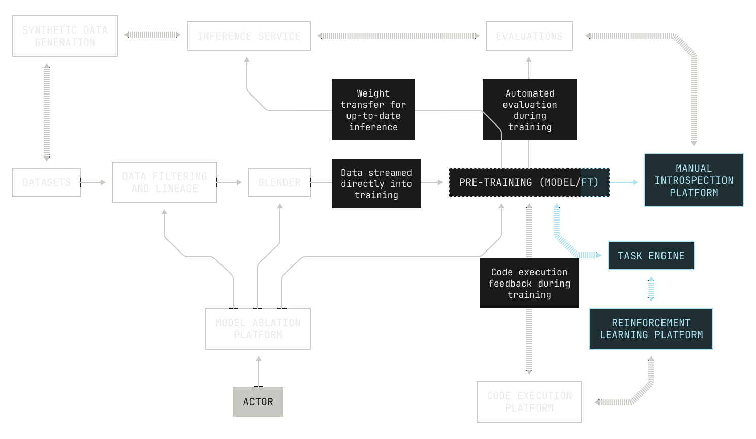
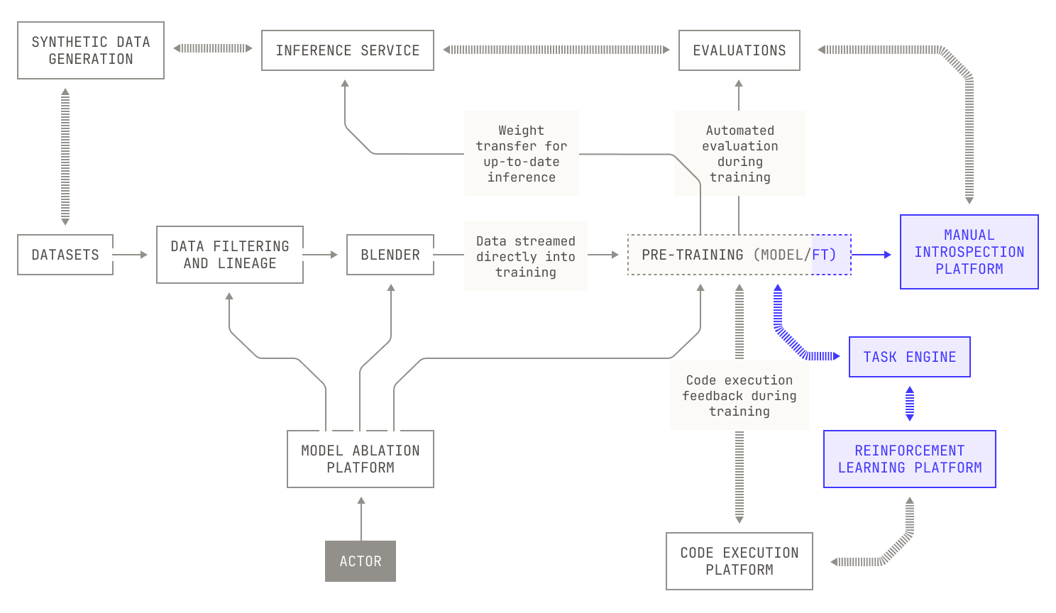
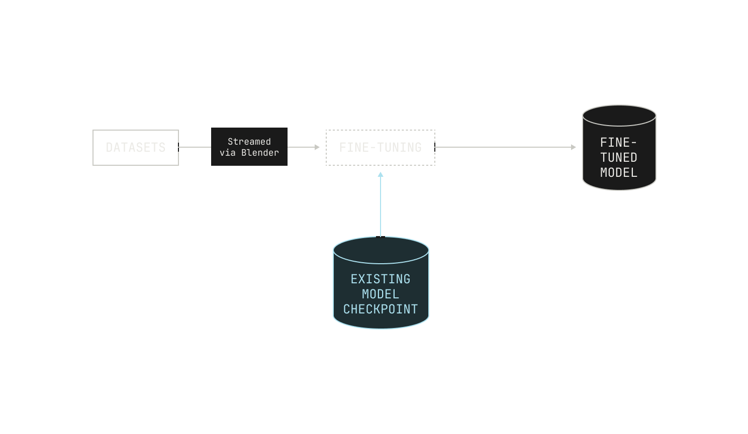
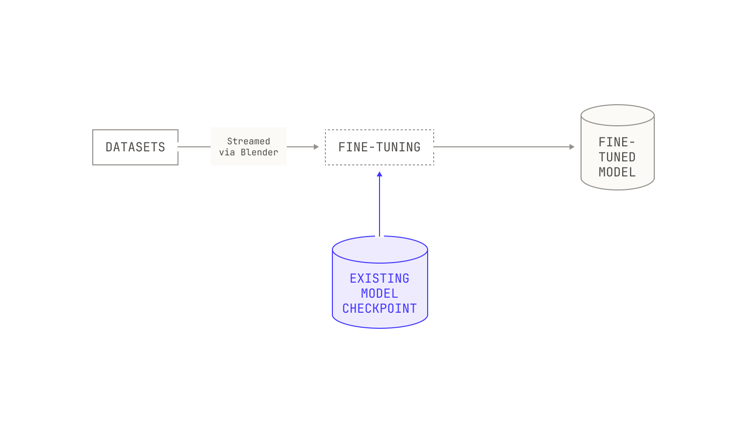
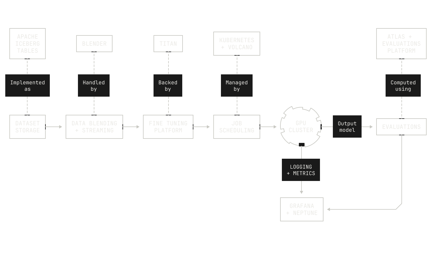
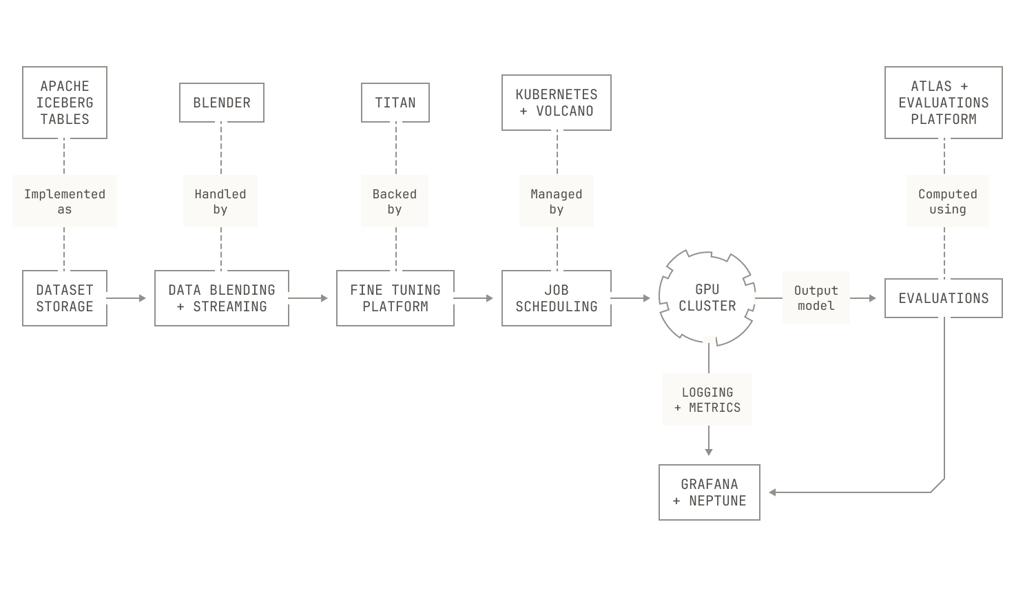
We’ll now consider our SFT workloads. As we mentioned earlier, SFT is very similar to pre-training: we stream a dataset into some training nodes, run a training-style workload, run automated evaluations, and ultimately store the newly produced checkpoint to a storage service. All of these steps are enabled by pieces of the Factory that we've introduced previously. Indeed, data streaming is enabled by our data blending and streaming platform (Blender); training is conducted using our distributed training codebase (Titan); and evaluations are handled by our broader evaluations system. We can even reuse our existing scheduling infrastructure to deploy SFT workloads. And the logistics of running experiments is similar to the rest of the Factory: our researchers can run new experiments simply by creating a new configuration file or forking an old one. Then, once they've settled on a configuration and merged it on Github, our CI runners automatically schedule and orchestrate the resulting jobs in Dagster. Of course, these workloads also make use of our other Model Factory tooling, like logging and metric streaming; and all job prioritization and scheduling is handled neatly by Volcano and Kubernetes. This all adds up to the following, high-level picture of how an SFT pipeline maps to Model Factory components:

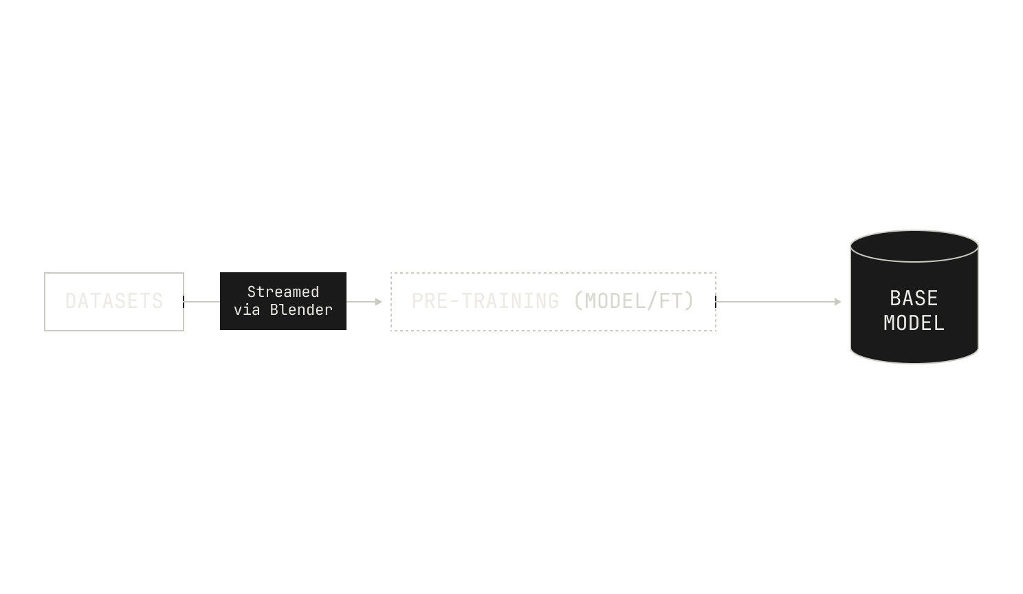
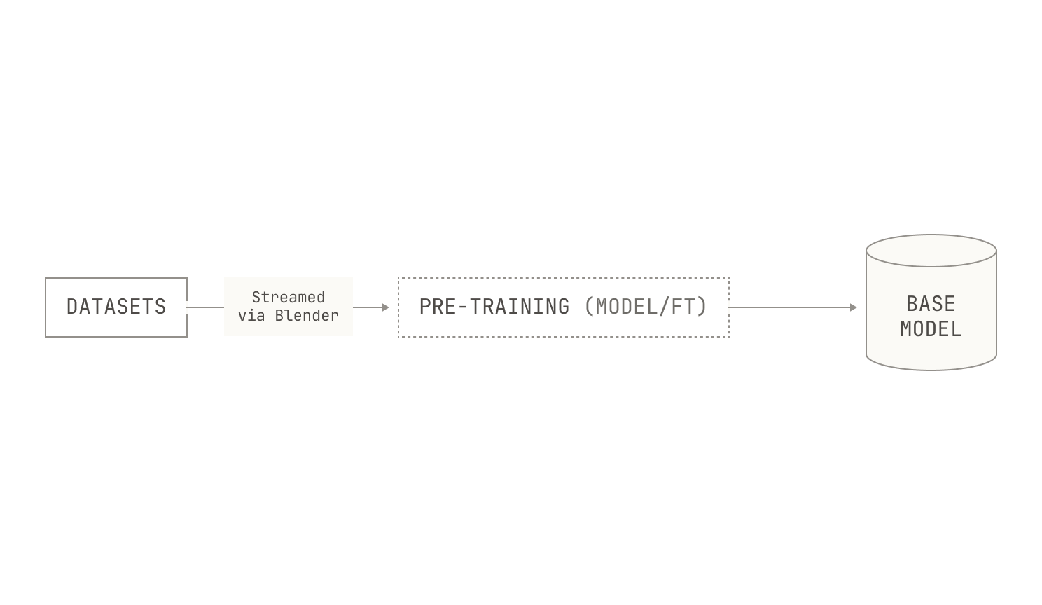
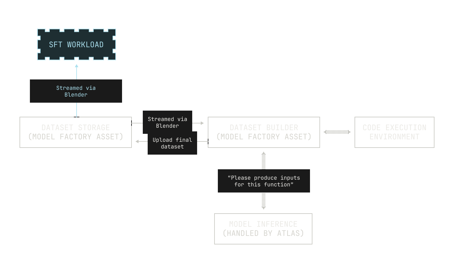
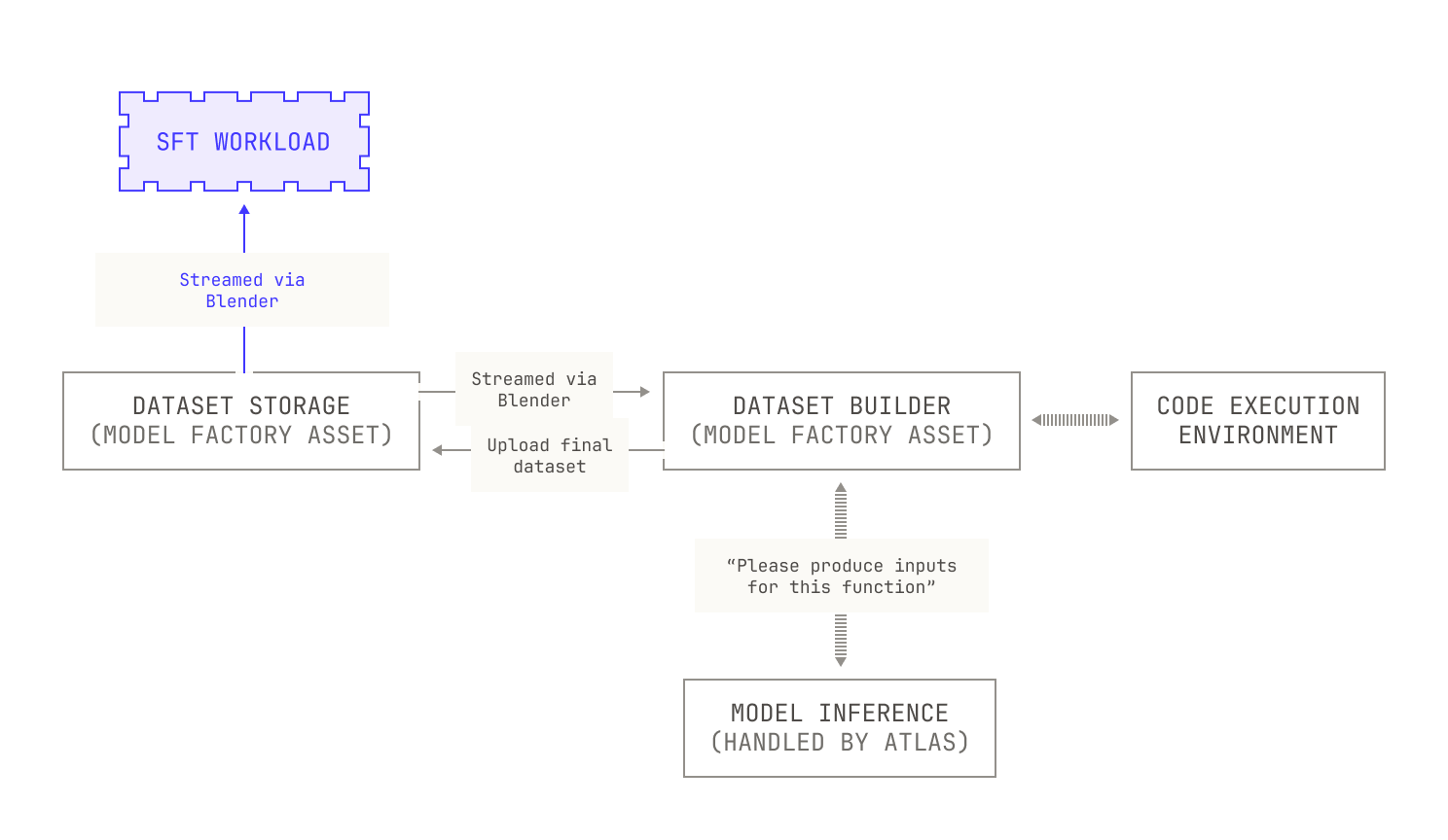
Of course, this only covers how we actually run SFT, and it doesn’t directly address how we can use the Model Factory to build datasets for SFT. As a motivating example, let's imagine that we want to conduct a small experiment on our model's ability to reason about code. To conduct this experiment, we'll build a static code execution dataset. In particular, our goal is to produce a dataset where each row contains a function definition, some sample inputs, and the result of calling the function with those inputs. To build such a dataset, we'll need a couple of things. First, we'll need some sample functions and some associated inputs (after all, without this we'll never be able to compute the outputs). For the sake of this example, we’ll imagine that we already have a sample function dataset, and we just need to come up with the inputs. In this case, we can deploy a model to handle this task for us: we’ll simply give a model a function definition and ask it to produce some valid arguments. Second, we need a way to actually compute the functions on the specified inputs. Visually speaking, this looks as follows:

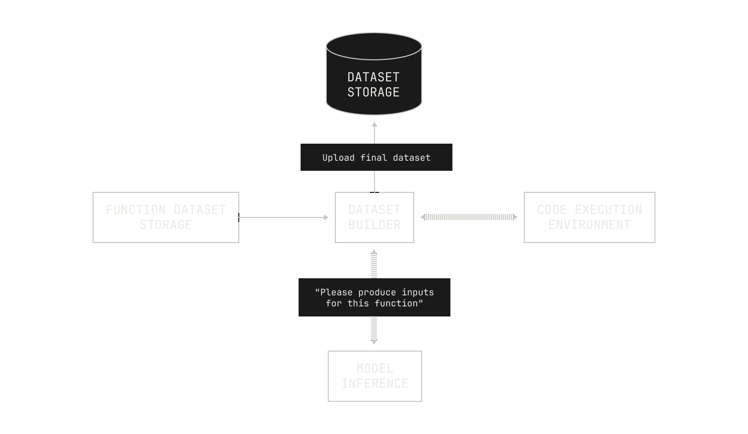
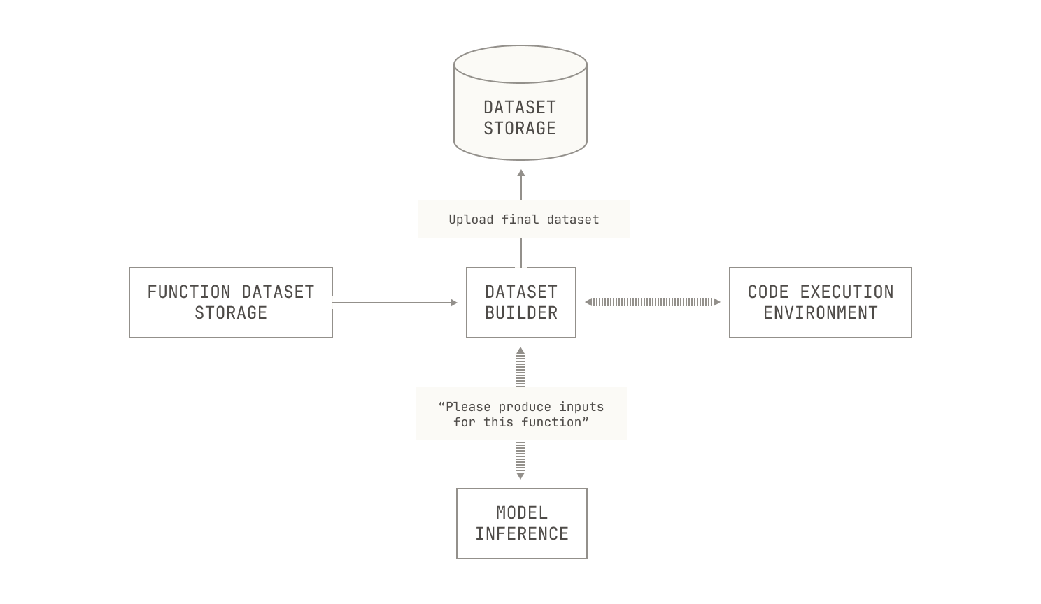
The Model Factory already has all of the pieces we need for dataset generation; we’ve introduced all of the pieces in our previous installments. First, we already know that the Model Factory supports reading and writing Apache Iceberg tables, so we can reuse these components to operate on our new datasets. We also know that the Model Factory has scalable services for both inference service and code execution, allowing us to produce this dataset easily. And when we actually use the dataset in fine tuning, we can use our Blender service to shuffle and stream the dataset onto our training nodes without requiring any extra handling. This leads to the following scenario:

Before we move on, we should note that because everything is tightly integrated in the Model Factory, any updates to upstream components automatically propagate throughout the Factory. For example, new parallelisms in Titan, or optimizations in Blender, influence almost every workflow in the Factory. And optimizations to workload-agnostic components (like our scheduling mechanisms) provide even greater improvements to our workflows, allowing us to further improve the efficiency of the Factory.

RL in the Model Factory

Our RL workloads also benefit from the broader maturity of the Model Factory. Indeed, although running RL workloads requires additional components compared to SFT—such as actor-critic loops, reward model infrastructure, and even asynchronous RL tooling—the remaining pieces are all present. This shouldn’t be a surprise: after all, the Model Factory acts as a general system for orchestrating complicated AI workloads, and post-training is simply a particular case. In fact, despite the differences between RL and SFT, the steps for running the experiments are the same: our researchers create new configuration files and build any new assets; then all we need to do is trigger the appropriate workflow in Dagster. Everything else, from scheduling to logging, is all handled by the components we’ve already introduced in the Model Factory.

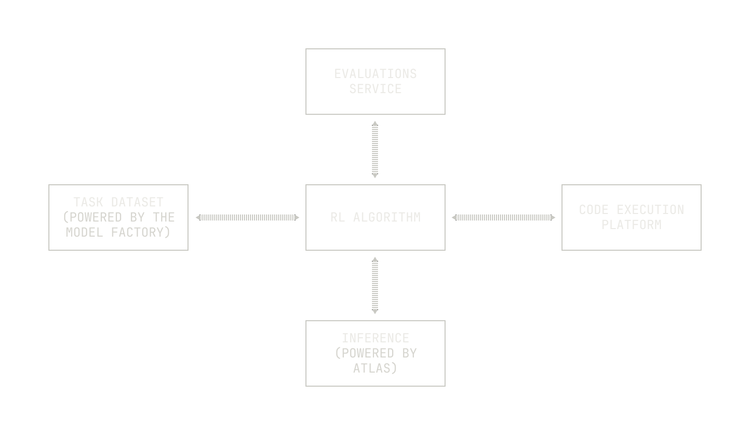
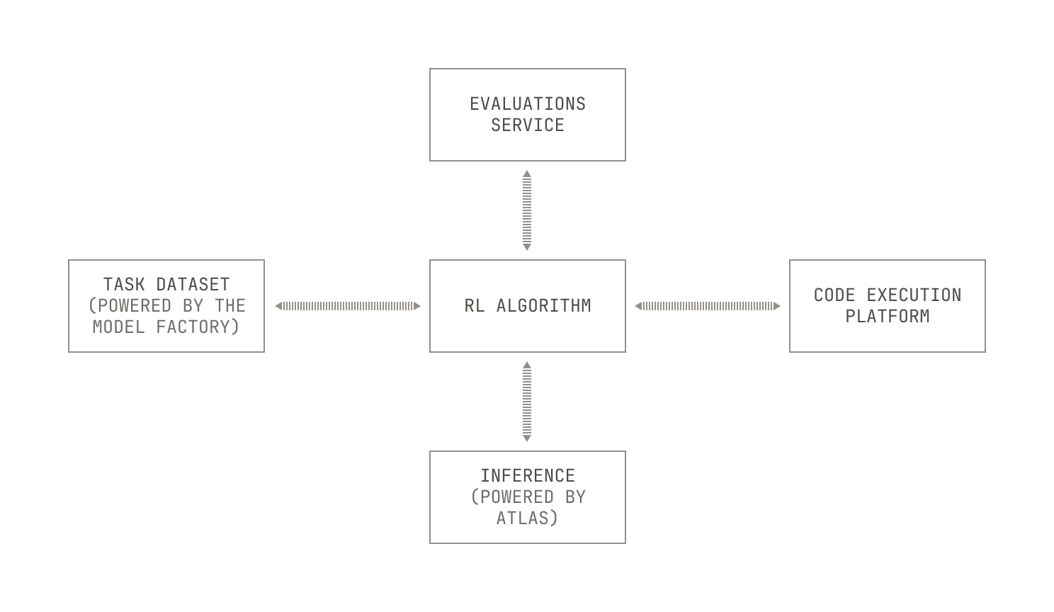
For the sake of example, we’ll discuss how we run RLCEF workloads. As a recap, RLCEF is our technique for teaching models how to solve various software engineering tasks and problems via reinforcement learning. We typically break RLCEF up into two components: an actor that solves tasks, and nodes that run training-style workloads. In more detail, our actors typically read input data from our data storage, and then attempt to solve tasks on the input data. The actors then learn using a reward mechanism and send their session transcript into Blender. Lastly, the training nodes read the session transcript from Blender, learning on the produced data.

This can be orchestrated as follows. First, we can see that both the actors and the training workflows need certain common components, like code execution and large-scale inference. We also, of course, need the job scheduling and task orchestration features from the Model Factory. And because we’re conducting a training workload too, we’ll also use Titan and our evaluations service. This leads to the following high-level picture:

Our earlier description is deliberately algorithm agnostic: we haven’t described any particular actor or RL algorithm for implementing RLCEF. This is because it doesn’t matter from an operations perspective: our researchers can simply implement a new RL or actor algorithm and it’ll automatically slot into the rest of the Factory.

Everything needed above is orchestrated and handled via our Dagster integrations, so all we need to do is implement the RL algorithms themselves. Practically speaking, we implement RL algorithms as standalone pieces inside the ModelFactory and simply specify which one we want to use as part of the experiment’s configuration file. In fact, the RL portion of the Model Factory has grown so large that it almost operates as its own “sub factory”: we have components for everything, from algorithms like GRPO and PPO through to actor-critic loops and various workload customizations. And each of these components is built around other, well-tested components in the Model Factory; for example, our RL actors all invoke code execution via our scalable Task Engine, allowing us to handle tens of millions of concurrent tasks at once.

In summary, the gains from being able to reuse Factory components can’t be overstated. Researchers and engineers at poolside don't spend their time manually running benchmarks or orchestrating data workflows; they spend their time thinking about how to improve poolside’s models. And, because the Model Factory is built as a scalable system, everything works—even if we have to swap out components. All we have to do is build the individual components that we need, and the rest of the Factory makes sure that everything just works.

Things we’ve built just for Post-training

Now that we’ve seen how the Model Factory can enable post-training, we’ll talk about some of the things that we’ve added to the Factory specifically for post-training. Before we get into the details, it’s worth highlighting that these components follow the same principles as the rest of the Factory, and none of the systems we discuss here are limited to post-training. In fact, the opposite is true: both of the components we’ll discuss here have already found practical use cases outside of post-training alone.

Podium, our dataset viewer

As mentioned previously, we spend a great deal of time at poolside manually inspecting fine tuning datasets in order to make sure that they're high quality. This is, in part, because it’s easy to introduce hard-to-spot bugs when generating a particular fine tuning dataset. For example, it’s fairly common to fine tune models to produce structured output, such as JSON or XML, but without proper tooling to inspect datasets, it’s quite easy to miss these bugs. Inspecting datasets also gives us further insights. For example, inspecting fine tuning datasets leads to good intuition about how to generate fine tuning datasets; indeed, by seeing which approaches to generation succeed, we can improve our ability to generate new datasets in the future. At the same time, inspecting datasets allows us to improve the dataset's quality: we get a strong feeling for which datasets are good and which ones are bad. This has a direct benefit: if we fine tune on a particular, high-quality dataset and the model's quality doesn't improve, then it must be the case that the fine tuning approach itself was flawed.

In order to inspect fine-tuning datasets, we've built an internal tool, called Podium. Podium allows researchers to load a particular dataset, generate new samples, and look at the results. Under the hood, Podium supports loading an entire Apache Iceberg table from our Dagster, giving us an unparalleled level of insight into our datasets. In practice, we've found that Podium helps us in three ways. First, Podium makes it straightforward to visualize complex datasets, allowing us to easily spot malformed samples and fix bugs. This is especially useful in the case of structured, or otherwise complicated, inputs and outputs. Second, Podium allows us to iterate over small datasets before we scale up generation; bluntly, there's no point in wasting large-scale compute on an approach that won't yield a good dataset. And lastly, Podium allows us to see how a model evolves over time: because we can generate new samples against any checkpoint, Podium makes it easy for us to see how our model evolves due to fine tuning.

Much like the rest of the Model Factory, Podium is now used for multiple, originally unintended uses. For example, we’ve recently extended Podium to support examining custom samples, allowing anyone involved in vibe checking to quickly supply prompts on which a particular model performs poorly. By extending Podium in this way, we’ve made it much easier to systematically gather subjective feedback on how our models perform; put differently, we’re able to more easily explain where we feel a particular model should improve. This also means we can easily build new internal evaluations, allowing us to build new core competencies into our models.

GPU<>GPU weight transfer

Before we conclude this series, let’s discuss one component of the Model Factory that sees extensive usage in RL workloads: GPU<>GPU weight transfer.

Recall that our RL workloads are typically split into two components: an actor component and a training component. Because we run these workloads at large scale, we necessarily need to run our RL workloads in an off-policy mode. However, given that off-policy RL can lead to poor quality models, we need a solution to quickly synchronize weights between nodes used for training and nodes used for acting. For the sake of this discussion, we’ll talk about weight synchronization in terms of moving weights between training and inference, since these are where fast synchronization is ultimately necessary.

First, we could use the same nodes for both training and inference, but this makes scaling difficult. Not only do we need to decide on the number of nodes for both training and inference at the same time, but we also can't independently scale either workload. If we increase the number of nodes for an inference workload, we also need to dedicate more nodes for training, regardless of whether we need them or not. Even if we were to somehow accept this limitation, we would also need to address the other issues that come with this approach. For instance, it’s not typical to have the same training and inference meshes, thus there’s no guarantee that every training node would have the right tensors to run inference on the same node without network activity. Of course, we can exchange tensors over the network via AllGather, but this would substantially impact training and lead to increased memory consumption. In other words, from the perspective of the Model Factory, co-locating inference and training is simply a non-starter.

Although we could reuse our large-scale storage systems from the Model Factory, there’s a more obvious approach. Intuitively, we’d like it if there were a way to simply transfer the weights from the GPUs that are used in training to the GPUs that are used for inference, without needing to use any intermediate steps. This approach—which we’ll call GPU<>GPU weight transfer—is already widely utilized in the RL community across various RL workloads. The difference, in our case, comes down to scale. In fact, for GPU<>GPU transfer to work for us, we would need to be able to transfer weights extremely quickly, as this is crucial to remaining as close to on-policy as possible. And, we want to be able to do this without any appreciable slowdown to either training or inference; otherwise, we simply won’t benefit from the increased performance.

To establish if GPU<>GPU transfer were something we could actually use in practice, we began to look at our P5e nodes more closely. For the unaware, P5e nodes are AWS EC2 instances equipped with 8 Nvidia H200 GPUs, and each P5e node provides a total of around 3200Gbps of network bandwidth via their EFAv3 networking fabric. Notably, P5e nodes also provide GPUDirect RDMA capabilities, which is a way for GPUs to quickly access each other's memory without requiring CPU involvement. This 3200Gbps of network bandwidth is substantial. After all, even Llama 405B stored in bfloat16 precision is only 810GB, so we could transfer all of the weights in around 2 seconds with full utilisation. This seems promising, but is it something we can actually use?

It turns out the answer is yes. We'll now describe how we did it.

First, the naive approach of co-locating training and inference requires executing an AllGather operation. AllGathers are very flexible, but there’s a better way. We just need to find a way to tell the GPUs that are involved in acting where they need to directly send their weights. The most simple case of this occurs when we want to do a one-to-one transfer. We can think of this scenario as sending from `n` GPUs on the left to `n` GPUs on the right: there's a precise one-to-one mapping between the weights.

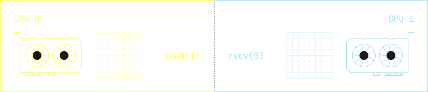
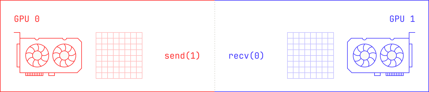
In this case, we can simply take advantage of NCCL's existing point-to-point primitives for transmitting data, and we just send data directly between devices. This, though, is the simplest possible case; after all, we might want to send from `n` GPUs on the left to `m` GPUs on the right. This could happen, for instance, if we want to experiment with quantized inference: we might require 2 GPUs for training, but only a single GPU for inference. If we zoom out slightly, we can even imagine situations where each GPU on the left needs to send a different chunk to each GPU on the right, requiring a much more complicated scheme.

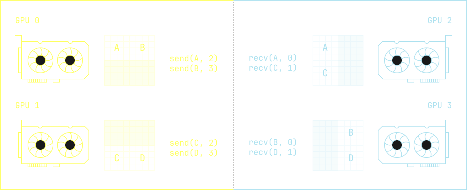
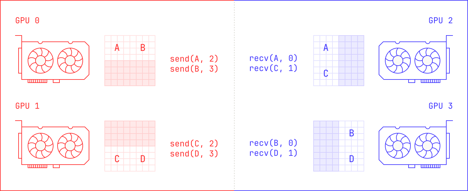
How do we solve this problem in general? The trick, it turns out, is to define an abstract topology that handles these details for us. Intuitively, we just need a way to tell any GPU on the left what it needs to send to every node on the right. This is a solved problem—MPI implementations have had support for similar techniques for years—but we still needed to implement such a scheme for NCCL. We note that implementing such an approach is quite complicated, even though it’s intuitively easy to explain. We need to handle the fact that both training and inference may have different meshes; there’s not necessarily a straightforward one-to-one mapping. In fact, sometimes different tensors need to be distributed in different ways. For instance, expert parallel tensors need to follow a different routing strategy to the tensors that make up the attention block. Moreover, even for the same scaling approach, such as tensor parallelism, we might use a different number of GPUs in fine tuning compared to inference. These details all add up to a lot of engineering work, but we finally have an approach that satisfies all of our criteria. Crucially, GPU<>GPU weight transfer now acts as just another machine in the Model Factory that we can use to achieve any number of tasks.

Even outside of typical engineering work, it's important to stress that implementing GPU<>GPU transfer is actually a remarkably complicated and brittle task, especially at our scale. From a software perspective, there's a strong need to ensure that all nodes in the cluster have the exact same software versions; even slight mismatches in, say, the NCCL library, can lead to hard-to-diagnose bugs and issues. Moreover, we regularly encountered deadlocks when implementing GPU<>GPU transfer. These deadlocks occurred for a variety of reasons, from mismatched send/recv order to resource contention across streams. For instance, we needed to add a warmup for all of the send & receive connections in NCCL because they would otherwise fail later on. Thankfully, we were able to resolve these issues, but at the cost of many hours of debugging. This point, in particular, is worth dwelling on: anecdotally, we noticed that debugging GPU<>GPU transfer had an unusually long feedback cycle. This is primarily due to scale. Indeed, we noticed that stability on a smaller collection of machines was not indicative of stability on a larger collection of machines, and thus we had to run many tests on thousands of GPUs. Given the failures were primarily non-deterministic, we spent a lot of time waiting for failures to occur before we could dig into them.

Before we conclude, we’ll discuss what GPU<>GPU transfer gives us in the context of the Model Factory. Metaphorically speaking, GPU<>GPU transfer is a conveyor belt between our training furnaces and our inference machines. Where before we would need to offload weights to a comparatively slow storage system, GPU<>GPU weight transfer now allows us to quickly move weights between fine tuning and inference. Notably, our implementation of GPU<>GPU weight transfer actually runs fully asynchronously, allowing us to continue training while we wait for the weights to arrive on the inference nodes. This efficient transfer is also extremely useful for other workloads: for instance, we could utilize GPU<>GPU weight transfer to quickly spin up new inference replicas on demand without requiring us to fetch model weights from a large-scale storage system. In fact, much like the rest of the Factory’s components, GPU<>GPU weight transfer should be viewed as just another piece of a larger, fully orchestrated system, and its uses are manifold.

Thank you

We hope you have enjoyed reading this post about how we conduct post-training inside the Model Factory. We also hope that you have enjoyed reading the broader Model Factory series; please check out the other posts if you haven’t already.

Interested in building machines for poolside's Model Factory? We'd love to hear from you.

→ View open roles

Acknowledgments

This series of posts has required input from almost every engineer at poolside. We would like to thank everyone for their thoughtful comments and insights on the posts; they’ve benefited tremendously from your comments. We would also like to thank the design team for their tireless work on the diagrams for this series. Lastly, we would like to thank the Dagster, Neptune and Grafana teams for their continued support and collaboration.